. 2017 Jul;29(7):2004-2020.
doi: 10.1162/NECO_a_00979. Epub 2017 May 31.

Analytical Derivation of Nonlinear Spectral Effects and 1/f Scaling Artifact in Signal Processing of Real-World Data

Affiliations

Analytical Derivation of Nonlinear Spectral Effects and 1/f Scaling Artifact in Signal Processing of Real-World Data

Claudia Lainscsek et al. Neural Comput. 2017 Jul.

Abstract

In estimating the frequency spectrum of real-world time series data, we must violate the assumption of infinite-length, orthogonal components in the Fourier basis. While it is widely known that care must be taken with discretely sampled data to avoid aliasing of high frequencies, less attention is given to the influence of low frequencies with period below the sampling time window. Here, we derive an analytic expression for the side-lobe attenuation of signal components in the frequency domain representation. This expression allows us to detail the influence of individual frequency components throughout the spectrum. The first consequence is that the presence of low-frequency components introduces a 1/f[Formula: see text] component across the power spectrum, with a scaling exponent of [Formula: see text]. This scaling artifact could be composed of diffuse low-frequency components, which can render it difficult to detect a priori. Further, treatment of the signal with standard digital signal processing techniques cannot easily remove this scaling component. While several theoretical models have been introduced to explain the ubiquitous 1/f[Formula: see text] scaling component in neuroscientific data, we conjecture here that some experimental observations could be the result of such data analysis procedures.


Figures

Figure 1
Figure 1
Effect of sub-cutoff frequency content (a) and linear drift (b) on spectral scaling. The fast Fourier transform (FFT) magnitude spectral estimate for a signal S1 = sin(2π f1t), where f1 = 10 Hz, fs = 1000 Hz, and T = 100 s, is given in black. (a) An additional signal S2 = sin(2π f2t) (f2 = 0.009 Hz), which is an arbitrary frequency smaller than the cutoff fc (in equation 1.3), is added to S1. (b) A linear drift S3=0.4Tt is added to S1. In both cases, the resulting spectral estimate is shown in magenta.
Figure 2
Figure 2
Analytical form of G(Ω)T for test frequencies F=Ω2π with several random phases φ and ϕ (red; see equation 2.15b) and derived envelopes (see equations 2.16). The width of E2 and E3 together is exactly the DFT bin length fc and is centered in the main lobe.
Figure 3
Figure 3
Error made for a single sinusoidal signal with a frequency of 10 Hz and sampling rate of 1000 Hz in the alternative representation (top) and for the Goertzel algorithm (middle). The difference (bottom) between both approaches, in percent of the signal amplitude, is small but nonvanishing. The light blue lines are the errors made for the different phases (Ω = ω; φ = ϕ = 0) in equation 2.15a, and the dark blue lines represent the sinc function (Ω = ω; φ = ϕ = 0).
Figure 4
Figure 4
Effect of the phase of the low-frequency component (fs = 1000 Hz, f = 0.009 Hz, and T=1fs) relative to the finite-length window. G(Ω)T is shown for phases between 0 and 2π as separate linear plots (top) and as polar plots where the logarithm of the frequency is plotted along the radius (bottom). The analytical form in equation 2.15b is shown on the left side and the numerical results for the Goertzel algorithm on the right side. The slope is −1 nearly everywhere. The slope is −2 only for φ=π(2n1)2, n ∈ ℕ. The dashed black lines (top plots) are the analytical form in equations 2.16.
Figure 5
Figure 5
Effect of the amplitude of the low-frequency component on the spectral scaling. FFT estimates of the frequency spectrum for varying amplitude of the 0.009 Hz (0.9 × fc) sub-cutoff frequency component. Amplitude of the sub-cutoff frequency added to the original 10 Hz sinusoid ranges from 0 (dark red) to 1 (blue); the original sinusoid is of unit amplitude. Note that the specific scaling component analyzed in the main text appears immediately on the addition of the low-frequency component at all amplitudes.
Figure 6
Figure 6
Effect of high-pass prefiltering on low-frequency intrusions. As in Figure 1, the FFT spectral estimates are given for an example 10 Hz sinusoid (black) and for the original signal with an added 0.009 Hz low-frequency component with random phase angle (magenta). Aversion of this composite signal filtered with a high-pass, 5000th-order, linear-phase FIR filter is plotted in turquoise.
Figure 7
Figure 7
Dependence of filtering on the phase of the sub-cutoff frequency component. The magnitude of slope for the spectral scaling is plotted as a polar function of the low-frequency phase for the original signal with an added 0.009 Hz low-frequency component (magenta) and for the signal filtered as in Figure 6 (turquoise). For this calculation, mean magnitude spectra were obtained by averaging over 100 trials at each phase using the Welch power spectral estimate, and fits were conducted on the smoothed results. The unit circle is plotted in black. Slope is determined by linear fit in log-log coordinates between 0.7 and 3 Hz, where the spectral scaling artifact is most prominent in the filtered version (see Figure 6). While the slope remains near −1 for the unfiltered signal, the slope of the filtered signal returns to zero only for angles close to φ=π(2n1)2, n ∈ ℕ.
Figure 8
Figure 8
Test with signal differencing. FFT spectral estimates for an example 10 Hz sinusoid (black), the same signal with added low-frequency component (blue), and this second signal preprocessed by differencing (red). The observed spectral scaling artifact remains in the differenced signal, illustrating the difficulty in removing this artifact through standard signal processing techniques.
Figure 9
Figure 9
Test with numerical detrending. (Left) A 10 Hz sinusoid with an added noisy oscillation (f(t) = A cos(ωt + η(t)), where η(t) represents frequency noise). The original signal is plotted in the top panel, and the detrended version is plotted at bottom. (Right) The spectra for the 10 Hz sinusoid (black), 10 Hz with added noisy, low-frequency component (magenta), and the detrended version of the composite signal (blue).
Figure 10
Figure 10
Test with numerical detrending under the influence of added white noise (SNR = 10 dB). (Left) A 10 Hz sinusoid with an added noisy oscillation (f(t) = (A + η1(t)) cos(ωt + η2(t)), where η1(t) and η2(t) represent amplitude and frequency noise, respectively). The original signal is plotted in the top panel, and the detrended version is plotted at bottom. (Right) The spectra for the 10 Hz sinusoid (black), 10 Hz with added noisy, low-frequency component (magenta), and the detrended version of the composite signal (blue).

References

    1. Cooley J, Lewis P, Welch P. The finite Fourier transform. IEEE Transactions on Audio and Electroacoustics. 1969;17(2):77–85.
    1. Erdélyi A, editor. Tables of integral transforms. Vol. 1. New York: McGraw-Hill; 1954.
    1. Fourier J. Thïéorie analytique de la chaleur. Chez Firmin Didot; 1822.
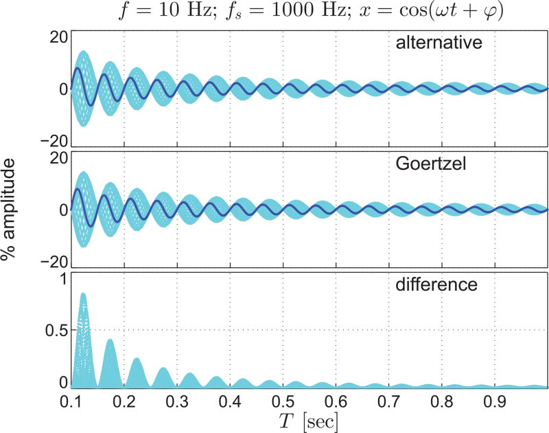
    1. Goertzel G. An algorithm for the evaluation of finite trigonometric series. American Mathematical Monthly. 1958;65(1):34–35.
    1. Harris FJ. On the use of windows for harmonic analysis with the discrete Fourier transform. Proceedings of the IEEE. 1978;66(1):51–83.

Publication types

LinkOut - more resources