Moran's I quantifies spatio-temporal pattern formation in neural imaging data

Abstract

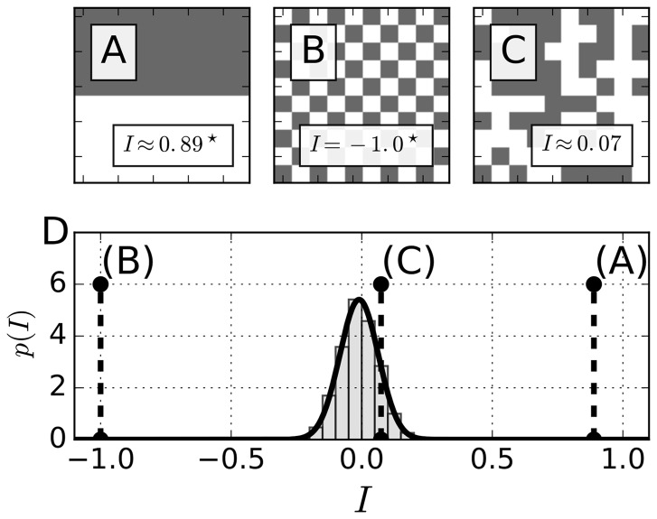
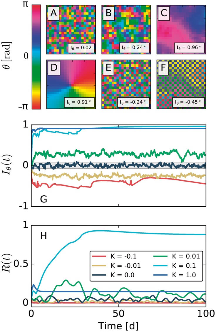
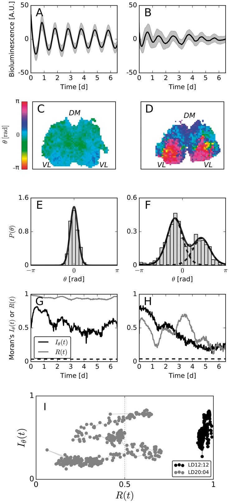
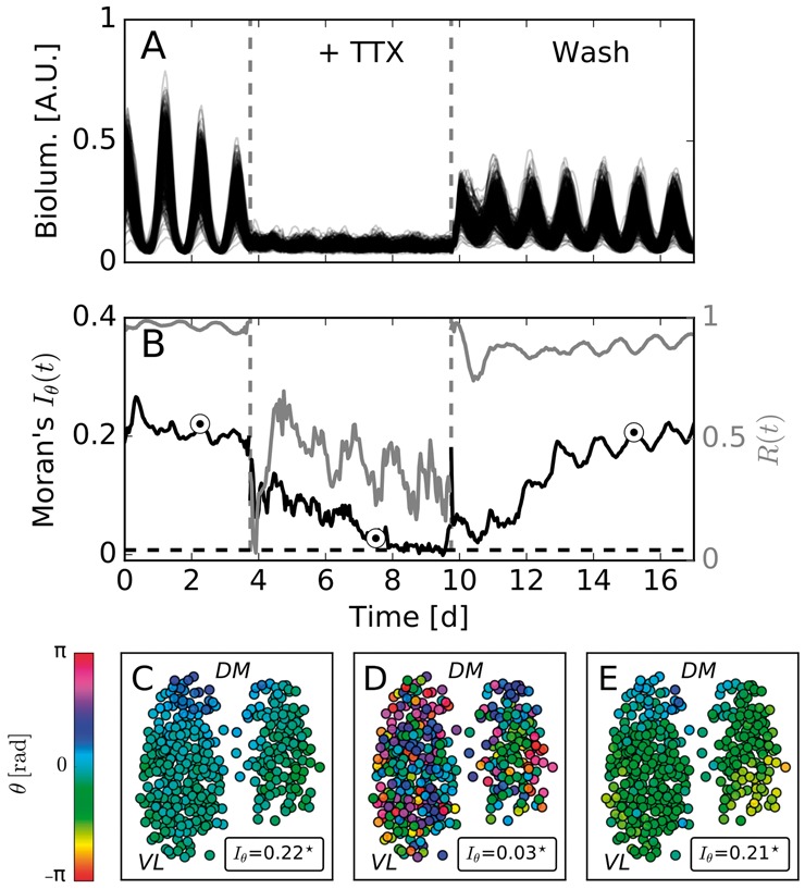
Motivation: Neural activities of the brain occur through the formation of spatio-temporal patterns. In recent years, macroscopic neural imaging techniques have produced a large body of data on these patterned activities, yet a numerical measure of spatio-temporal coherence has often been reduced to the global order parameter, which does not uncover the degree of spatial correlation. Here, we propose to use the spatial autocorrelation measure Moran's I, which can be applied to capture dynamic signatures of spatial organization. We demonstrate the application of this technique to collective cellular circadian clock activities measured in the small network of the suprachiasmatic nucleus (SCN) in the hypothalamus.

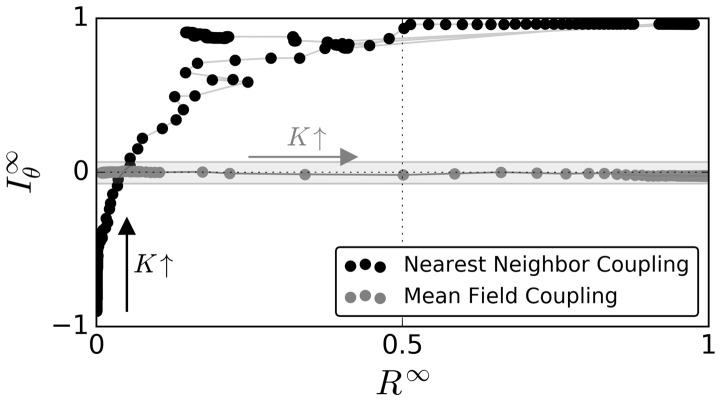
Results: We found that Moran's I is a practical quantitative measure of the degree of spatial coherence in neural imaging data. Initially developed with a geographical context in mind, Moran's I accounts for the spatial organization of any interacting units. Moran's I can be modified in accordance with the characteristic length scale of a neural activity pattern. It allows a quantification of statistical significance levels for the observed patterns. We describe the technique applied to synthetic datasets and various experimental imaging time-series from cultured SCN explants. It is demonstrated that major characteristics of the collective state can be described by Moran's I and the traditional Kuramoto order parameter R in a complementary fashion.

Availability and implementation: Python 2.7 code of illustrative examples can be found in the Supplementary Material.

Contact: christoph.schmal@charite.de or grigory.bordyugov@hu-berlin.de.

Supplementary information: Supplementary data are available at Bioinformatics online.

Fig. 1.

Moran’s I detects non-random spatial patterns. (A–C) Illustrative examples of spatial distributions on a binary 10 × 10 grid where each grid cell either adopts a value of 0 (white) or 1 (gray). D) Distribution of all possible values of I on a 10 × 10 grid conditioned to a von Neumann neighborhood of range r = 1. The histogram was obtained by determining I for $N={10}^6$ randomly generated patterns under the assumption of an unbiased probability of occurrence of the binary values. The bold black line denotes a fit of a normal distribution to the data, resulting in $\mu \approx -0.01$ and $\sigma \approx 0.07$. Dashed black lines highlight the specific indices I determined for the patterns in panels (A)–(C)

Fig. 2.

Moran’s $I_{\theta }$ reliably detects spatial ordering in the phase dynamics of a two-dimensional array of coupled Kuramoto phase oscillators with nearest neighbor interactions. (A–F) Spatial phase distributions at time $t=100\hspace{0.17em}\mathrm{d}$ for different values of coupling strength K but identical distributions of initial conditions and intrinsic periods that were sampled from a uniform as well as a normal distribution, respectively. The corresponding coupling strengths K in panels (A-F) are $K=0,0.01,0.1,1,-0.01,-0.1$, respectively. G-H) Dynamical evolution of Moran’s index $I_{\theta }(t)$ and the phase coherence R(t). Note that $I_{\theta }(t)$ and R(t) correspond to the same simulations that lead to the phase distributions at $t=100$ d as represented in panels (A-F). The gray-shaded area depicts the range of $I_{\theta }$ values for which the null hypothesis of no spatial autocorrelation cannot be withdrawn at a significance level 0.05 with a two-sided test. The corresponding sampling distribution is depicted in Supplementary Figure S3

Fig. 3.

Time averages of steady-state dynamics (i.e. after the decay of transient dynamics) of Moran’s index ($I_{\theta }^{\infty }$) plotted versus the steady state global phase coherence ($R^{\infty }$) for different coupling strength $K\in [-0.2,1]$, either for the case of nearest neighbor couplings (black dots) or a global mean field coupling (gray dots). Details on the numerical calculation of steady state values can be found in the caption of Supplementary Figure S1. Each dot corresponds to one particular simulation for a given coupling strength K. Lines connect dots that correspond to experiments sharing the smallest differences in coupling strength K. Black and gray arrows denote the direction of increasing coupling strength K in case of nearest-neighbor and mean-field couplings, respectively. The gray-shaded area depicts the range of $I_{\theta }$ values for which the null hypothesis of no spatial autocorrelation cannot be withdrawn at a significance level 0.05 with a two-sided test, similar to Figure 2

Fig. 4.

(A, B) PER2::LUC expression, averaged over all grid elements that contain SCN tissue (bold black lines), and the corresponding standard deviations (gray shaded area) for each SCN tissue after equinoctial (A) or long-day (B) entrainment. (C, D) Color-coded instantaneous phases ${\left\{{\theta }_t\right\}}_i$ at time $t=20$ h of the equinox (C) or long-day (D) entrained tissue. The abbreviations DM and VL indicate rough positions of the dorso-medial and ventro-lateral regions of the SCN, respectively. (E, F) Zero-centered histogram of the phase values as depicted in (C) and (D), respectively. (G, H) Dynamical evolution of R(t) (gray bold line) as well as $I_{\theta }(t)$ (black bold line) in case of equinox (G) and long-day (H) entrainment. Dashed black lines correspond to the upper critical values of I, estimated computationally from the sampling distribution as described in Section 2.6 at a significance level of 0.05 using a two-sided test. Corresponding sampling distributions are depicted in Supplementary Figure S4. (I) Dynamical evolution of Moran’s index and the global phase coherence in the $I_{\theta }(t)-R(t)$ plane. Bold lines connect two circles of $(R(t),I_{\theta }(t))$ tuples subsequent to each other

Fig. 5.

Suspension of synaptic couplings decreases the degree of spatial order in clock gene expression dynamics: (A) Bioluminescence time series. (B) Moran’s index $I_{\theta }(t)$ (bold black line) and mean-field phase coherence R(t) (bold gray line) for the time series plotted in the panel (A). (C–E) Color coded instantaneous phases ${\theta }_i(t)$ estimated by means of a Hilbert transform. Plotted phase distributions correspond to the time instances depicted by circles in the panel (B). Stars denote statistically significant deviations from the null hypothesis of no spatial autocorrelation. The abbreviations DM and VL indicate rough positions of the dorso-medial and ventro-lateral regions of the SCN, respectively. The dashed black line in (B) corresponds to the upper critical value of $I_{\theta }$, as described in Figure 4. The corresponding sampling distribution is depicted in Supplementary Figure S5

References

1. Abel J.H. et al. (2016) Functional network inference of the suprachiasmatic nucleus. Proc. Natl. Acad. Sci. USA, 113, 4512–4517. - PMC - PubMed
1. Acebrón J.A. et al. (2005) The Kuramoto model: a simple paradigm for synchronization phenomena. Rev. Mod. Phys., 77, 137–185.
1. Aton S.J., Herzog E.D. (2005) Come together, right…now: synchronization of rhythms in a mammalian circadian clock. Neuron, 48, 531–534. - PMC - PubMed
1. Aton S.J. et al. (2005) Vasoactive intestinal polypeptide mediates circadian rhythmicity and synchrony in mammalian clock neurons. Nat. Neurosci., 8, 476–483. - PMC - PubMed
1. Azzi A. et al. (2017) Network dynamics mediate circadian clock plasticity. Neuron, 93, 1–10. - PMC - PubMed