Modeling elucidates how refractory period can provide profound nonlinear gain control to graded potential neurons

Abstract

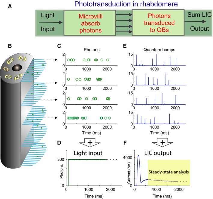
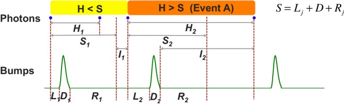
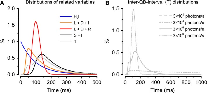
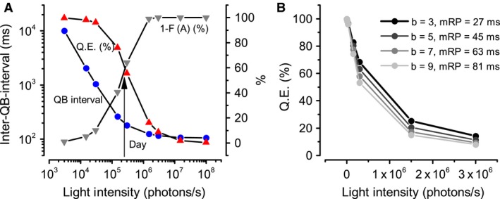
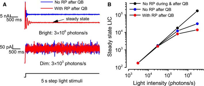
Refractory period (RP) plays a central role in neural signaling. Because it limits an excitable membrane's recovery time from a previous excitation, it can restrict information transmission. Classically, RP means the recovery time from an action potential (spike), and its impact to encoding has been mostly studied in spiking neurons. However, many sensory neurons do not communicate with spikes but convey information by graded potential changes. In these systems, RP can arise as an intrinsic property of their quantal micro/nanodomain sampling events, as recently revealed for quantum bumps (single photon responses) in microvillar photoreceptors. Whilst RP is directly unobservable and hard to measure, masked by the graded macroscopic response that integrates numerous quantal events, modeling can uncover its role in encoding. Here, we investigate computationally how RP can affect encoding of graded neural responses. Simulations in a simple stochastic process model for a fly photoreceptor elucidate how RP can profoundly contribute to nonlinear gain control to achieve a large dynamic range.

Keywords: Drosophila; fly photoreceptor; large dynamic range; neural adaptation; quantal sampling; quantum bump; stochasticity; vision.

Figure 1

Fly phototransduction model schematic. (A) The phototransduction takes place in the rhabdomere, which transduces light input (a dynamic flux of photons) into macroscopic output, light‐induced current (LIC). (B) The rhabdomere contains 30,000 microvilli (blue bristles), acting as photon sampling units. (C) Photons are randomly distributed over the 30,000 microvilli. Because of the large microvillus population, each of them will only absorb a photon sequence, which can be approximated by a Poisson point process (each row of open circles indicate a photon sequence absorbed by a single microvillus over time). (D) The light input (green trace) can be reconstructed by adding up all the photons distributed across the 30,000 microvilli. (E) The successfully absorbed photons in each microvillus are transduced into QBs (a row of QB events). In each microvillus, the success of transducing a photon into a QB depends upon whether the microvillus is in its refractory state. The photons hitting a refractory microvillus cannot evoke QBs, but will be lost. (F) QBs from all the microvilli integrate the dynamic macroscopic LIC.

Figure 2

Schematic of photon sequence and QB sequence in a microvillus. H denotes the photon arrival intervals. L is the latency in converting a photon to a QB and R is the refractory period after a QB. D is the bump duration and S the minimum inter‐QB‐intervals, i.e. any photons that arrive during S will be lost. S can be calculated as the summation of L, D and R. I is the waiting time for the next photon arrival. Depending the relationships between H and S, inter‐QB‐intervals, T, can be approximated by different quantities. If Hk>Sk, then Tk = Hk or Tk Lk + Dk + Ik, otherwise, Tk = Sk+Ik.

Figure 3

Inter‐QB‐interval distributions. (A) Probability distributions for different random variables defined. Both the photon intervals, H, and the next photon arrival waiting time, I, follow exponential distributions (blue line). L + D + I is the inter‐QB‐interval without a refractory period, but with a constraint that another QBcannot be excited before a QB termination (orange line). S = L + D + R adds the physical constraint in QB generation; a second QB can only be triggered after the first QB's refractory period (red line). If photon arrival statistics is considered, S + I is the inter‐QB‐interval at bright light conditions (black line). Finally, the p.d.f. of inter‐QB‐intervals, T, is the weighted sum from the distributions of L + D + I and S + I. Because of this weighted operation, a hump emerges in T's p.d.f. at small inter‐QB‐intervals (light grey line). (B) Adaptation takes place in inter‐OB‐interval distributions at different light intensities.

Figure 4

Inter‐QB‐intervals and QE adapt with brightening. (A) With increased contribution from refractory period (grey), the inter‐QB‐interval and QE reduces nonlinearly with brightening (blue and red). In dim light conditions, the mean photon arrival intervals can approach to 10 sec, which is much longer than the mean RPs (~100 msec). In these cases, refractory period contributes minimal, and QE approaches 100%. As light intensity increases, inter‐QB‐interval drops roughly linearly until an intensity that matches the population QB rate (QB rate/microvillus x #microvilli). In this particular case for a Drosophila photoreceptor, this light intensity is 3 × 10⁵ photons/sec, replicating living room day light conditions. It is also at this light condition that RP start to play an important role in tuning the system's gain (contributions over 50%), leading a sharp drop in the QE. As it becomes brighter, inter‐QB‐interval approaches to its limit, where RP is the dominating factor (>90%). The QE drops to 8% at the outdoor overcast light intensity (3 × 10⁶ photons/sec). When the light intensity increases to 1 × 10⁶ photons/sec (bright daylight), the QE can even drop to 0.26%. (B) The reduction rate of QE versus brightening is highly dependent on the statistical properties of refractory periods. We only tuned parameter b for the gamma distribution of refractory periods, and kept parameter “a” the same as shown in Table 1. With increasing b, the mean of refractory periods (mRP) increases, and the rate of QE reduction goes up.

Figure 5

Comparison of steady state LIC, modeled with and without RP. (A) Simulated LIC with and without RP after QB. 5 sec light step was the input (bottom), and the mean steady state LIC the output. In dim light (middle), RP plays no role, and the LICs with and without RP have similar amplitudes. In bright light (top), RP reduces the steady state response by half, tuning the system gain nonlinearly. (B) If all photons were converted to a stereotyped QB, the Intensity‐LIC relationship would be linear (black). However, with photons lost during the QB, the intensity‐LIC relationship reduces at bright conditions (blue). With a further RP after QB, the gain reduces more with brightening (red).

References

1. Adrian, E. D. , Zotterman Y.. 1926. The impulses produced by sensory nerve‐endings: Part II. The responses of a single end‐organ. J. Physiol. 61:151–171. - PMC - PubMed
1. Avissar, M. , Wittig J. H., Saunders J. C., and Parsons T. D.. 2013. Refractoriness enhances temporal coding by auditory nerve fibers. J. Neurosci. 33:7681–7690. - PMC - PubMed
1. Berry, M. J. , and Meister M.. 1998. Refractoriness and neural precision. J. Neurosci. 18:2200–2211. - PMC - PubMed
1. Blomfield, S. 1974. Arithmetical operations performed by nerve‐cells. Brain Res. 69:115–124. - PubMed
1. Brette, R. 2015. Philosophy of the spike: rate‐based vs. spike‐based theories of the brain. Front. Syst. Neurosci. 9:1–14. - PMC - PubMed
MeSH terms
LinkOut - more resources