Expansion of the Lyme Disease Vector Ixodes Scapularis in Canada Inferred from CMIP5 Climate Projections

Abstract

Background: A number of studies have assessed possible climate change impacts on the Lyme disease vector, Ixodes scapularis. However, most have used surface air temperature from only one climate model simulation and/or one emission scenario, representing only one possible climate future.

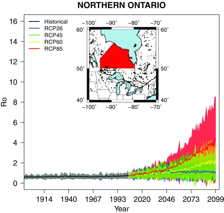
Objectives: We quantified effects of different Representative Concentration Pathway (RCP) and climate model outputs on the projected future changes in the basic reproduction number (R₀) of I. scapularis to explore uncertainties in future R₀ estimates.

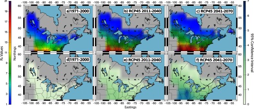
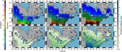
Methods: We used surface air temperature generated by a complete set of General Circulation Models from the Coupled Model Intercomparison Project Phase 5 (CMIP5) to hindcast historical (1971-2000), and to forecast future effects of climate change on the R₀ of I. scapularis for the periods 2011-2040 and 2041-2070.

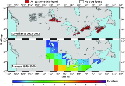
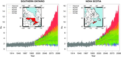
Results: Increases in the multimodel mean values estimated for both future periods, relative to 1971-2000, were statistically significant under all RCP scenarios for all of Nova Scotia, areas of New Brunswick and Quebec, Ontario south of 47°N, and Manitoba south of 52°N. When comparing RCP scenarios, only the estimated R₀ mean values between RCP6.0 and RCP8.5 showed statistically significant differences for any future time period.

Conclusion: Our results highlight the potential for climate change to have an effect on future Lyme disease risk in Canada even if the Paris Agreement's goal to keep global warming below 2°C is achieved, although mitigation reducing emissions from RCP8.5 levels to those of RCP6.0 or less would be expected to slow tick invasion after the 2030s. https://doi.org/10.1289/EHP57.

Figure 1.

Top: Data from active tick surveillance conducted between both 2003–2012 (Bouchard et al. 2015) and 2008–2013 (Ogden et al. 2014a). Locations where at least one I. scapularis tick has been found are marked by red triangles. White triangles mark locations where no I. scapularis ticks were collected. Bottom: Historical multimodel mean ${\mathrm{R}}_0$ estimates for the period 1971–2000. The ${\mathrm{R}}_0$ bar provides a color gradient showing the colors, which correspond to specific ${\mathrm{R}}_0$ values. The numbers around both the top and bottom maps depict the northings and eastings associated with the domain.

Figure 2.

Multimodel mean ${\mathrm{R}}_0$ values for I. scapularis (maps a−c) and the climate model variability (95% confidence interval) (maps d−f) for the period 1971–2000 using the historical simulation and for the periods 2011–2040 and 2041–2070 using RCP4.5 simulations. ${\mathrm{R}}_0>1$ values were mapped for areas east of the Rocky Mountains and for elevations below 500 m. The ${\mathrm{R}}_0$ bar provides a color gradient showing the colors, which correspond to specific ${\mathrm{R}}_0$ values. The numbers around the maps depict the Northings and Eastings associated with the domain. Black stippling in maps b and c shows the spatial distribution of statistically significant changes in ${\mathrm{R}}_0$ between each future time period (2011–2040 and 2041–2070) and the historical time period (1971–2000). Statistical significance was calculated using the Kolmogorov-Smirnov test.

Figure 3.

Multimodel mean ${\mathrm{R}}_0$ values for I. scapularis (maps a−c) and the climate model variability (95% confidence interval) (maps d−f) for the period 1971–2000 using the historical simulations and for the periods 2011–2040 and 2041–2070 using RCP8.5 simulations. ${\mathrm{R}}_0>1$ values were mapped for areas east of the Rocky Mountains and for elevations below 500 m. The ${\mathrm{R}}_0$ bar provides a color gradient showing the colors, which correspond to specific ${\mathrm{R}}_0$ values. The numbers around the maps depict the Northings and Eastings associated with the domain. Black stippling in maps b and c shows the spatial distribution of statistically significant changes in ${\mathrm{R}}_0$ between each future time period (2011–2040 and 2041–2070) and the historical time period 1971–2000. Statistical significance was calculated using the Kolmogorov-Smirnov test.

Figure 4.

Annual estimates of the ${\mathrm{R}}_0$ multimodel mean and the climate model variability (95% confidence interval) for Ontario south of 50°N (left) and Nova Scotia (right).

Figure 5.

Annual estimates of the ${\mathrm{R}}_0$ multimodel mean and the model variability (95% confidence interval) for Ontario north of 50°N.

References

1. Adrion ER, Aucott J, Lemke KW, Weiner JP. 2015. Health care costs, utilization and patterns of care following Lyme disease. PLoS ONE 10:e0116767, PMID: 25650808, 10.1371/journal.pone.0116767. - DOI - PMC - PubMed
1. Baldwin DJB, Desloges JR, Band LE. 2001. Physical geography of Ontario. In: Ecology of a Managed Terrestrial Landscape: Patterns and Processes of Forest Landscapes in Ontario, Perera AH, Euler DL, Thompson ID, eds. Vancouver: UBC Press, 12–29.
1. Bouchard C, Leonard E, Koffi JK, Pelcat Y, Peregrine A, Chilton N, et al. 2015. The increasing risk of Lyme disease in Canada. Can Vet J 56(7):693–699, PMID: 26130829. - PMC - PubMed
1. Buis A. 2011. Climate change may bring big ecosystem changes. http://climate.nasa.gov/news/645/ [accessed 1 December 2015].
1. Bush EJ, Loder JW, Mortsch LD, Cohen SJ. 2014. An overview of Canada's changing climate In: Canada in a Changing Climate: Sector Perspectives on Impacts and Adaptation, Warren FJ, Lemmen DS, eds. Ottawa: Government of Canada, 23–64.
Publication types
LinkOut - more resources