The energy landscape underpinning module dynamics in the human brain connectome

Abstract

Human brain dynamics can be viewed through the lens of statistical mechanics, where neurophysiological activity evolves around and between local attractors representing mental states. Many physically-inspired models of these dynamics define brain states based on instantaneous measurements of regional activity. Yet, recent work in network neuroscience has provided evidence that the brain might also be well-characterized by time-varying states composed of locally coherent activity or functional modules. We study this network-based notion of brain state to understand how functional modules dynamically interact with one another to perform cognitive functions. We estimate the functional relationships between regions of interest (ROIs) by fitting a pair-wise maximum entropy model to each ROI's pattern of allegiance to functional modules. This process uses an information theoretic notion of energy (as opposed to a metabolic one) to produce an energy landscape in which local minima represent attractor states characterized by specific patterns of modular structure. The clustering of local minima highlights three classes of ROIs with similar patterns of allegiance to community states. Visual, attention, sensorimotor, and subcortical ROIs are well-characterized by a single functional community. The remaining ROIs affiliate with a putative executive control community or a putative default mode and salience community. We simulate the brain's dynamic transitions between these community states using a random walk process. We observe that simulated transition probabilities between basins are statistically consistent with empirically observed transitions in resting state fMRI data. These results offer a view of the brain as a dynamical system that transitions between basins of attraction characterized by coherent activity in groups of brain regions, and that the strength of these attractors depends on the ongoing cognitive computations.

Keywords: Community structure; Energy landscape; Functional brain network; Graph theory; Maximum entropy model; Modularity.

Fig. 1

Schematic of local community allegiance energy landscape estimation. (A) Fluctuations of the strength of functional connectivity between brain regions over time manifests as reconfiguration of the brain’s functional modules. (B) The state of the community allegiance of a single region (e.g., node A) with the rest of the brain regions (‘1’ when both pairs appear in the same community (yellow nodes) and ‘0’ otherwise (blue nodes)) are then used to establish local functional module allegiance states. (C) We fit a MEM using these allegiance state vectors and estimate the functional interaction strength between brain regions to construct an energy landscape of regional community allegiance states.

Fig. 2

Local Minima in the Brain’s Functional Energy Landscape. (A) We identified M = 25 unique local minima states characteristic of the time series of a region’s allegiance to putative functional modules over time. Here, each state represents the set of regions that are commonly allied together in a single community. Using hierarchical clustering, we identified three classes of ROIs with similar patterns of community allegiance across these local minima. Class-I (blue), Class-II (red), and Class-III (green) branches are shown in the dendrogram on the right side of the matrix and visualized on the brain images as ROIs. Using the same clustering technique applied to the matrix transpose, we identified several classes of minima states with common ROI members, denoted by the colored branches on the top of the matrix. ICN labels and their corresponding Lausanne atlas ROI are provided in Table 1. (B) In addition to identifying the unique minima states, for each ROI we also calculated the basin size of local minima states as the fraction of the number of basin states to the number of total possible states. Note that the sizes of the analogous basins slightly vary across some ROIs since each local energy landscape is estimated using only 9 out of the 10 ROIs. (C) Calculating the Pearson correlation coefficient between any two ROIs’ vectors of basin size across minima states revealed groups of ROIs with similar energy landscapes. (D) The basin states’ average vectors highlight the unifying features of the basin states, i.e. omni-present core ROIs (average value 1), commonly present core ROIs (average value between 0.5 and 1) that tend to be among the minima states’ member ROIs, and finally the ROIs with incongruent membership (average value <0.5). (E) The average dwell time of minima state’s basins (all ROIs combined) grows exponentially with respect to the basins’ size. The close exponential fit (red curve) highlights this relationship.

Fig. 3

Empirically Estimated Transition Frequncies Between Basins. (A) The circular graph represents the empirical basin transition frequency pattern of a sample Class-II ROI representing the left hemisphere executive control network (LECN). Each color coded dot along the circumference of the circular graph represents one of the 25 local minima states. Lines linking local minima states indicate empirically estimated transition frequencies between local minima states’s basins; the width of the line is proportional to the empirically estimated frequency of that transition. The length of the lines and the width of the vertical colored bars contain no quantitative information and they serve only to enhance the visualization of the connected minima states. Transition frequencies are separately normalized for ROIs by dividing by the largest transition frequencies calculated for each ROI. All ICNs with community allegiance congruent with LECN (red overlay) are represented with yellow brain overlays (z > 1.5) for all 4 local minima states. (B) The empirical basin transition frequency pattern for two sample ROIs from Class-I (Visual) and Class-III (DMN). Note that unlike LECN, the basin transition frequency pattern of the visual ROI is heavily skewed towards a single state (that is, state 17, which we describe in greater detail in the body of the text).

Fig. 4

Empirical versus predicted frequencies of transitioning between basins. (A) We used a Markov Chain Monte Carlo (MCMC) simulation over the energy landscape of each ROI via the Metropolis-Hastings algorithm to estimate theoretically predicted frequencies of transitioning between basins of local community allegiance dynamics of ROIs. The normalized empirical and model transition frequencies were significantly correlated for Class-I(left) and Class-III (middle) ROIs but not for Class-II(right) ROIs. Colored dots represent values on the lower (red) and upper (blue) triangles of the transition matrices (See SI2 for details). The β-value represents the slop of the fitted line, the p-value represents the significance of the fit, and R² represents the corrected R² values for all of the regressions (B) We define the net empirical basin transition frequencies of minima states as the total in and out transition frequencies. These net frequencies are strongly correlated with the size of the basin surrounding each minima state, particularly for Class-I and Class-III ROIs. (C) Relationship between the empirical basin transition frequency and the predicted energy barriers estimated from a symmetrized transition frequency matrix. (D) Relationship between the empirical basin transition frequency and the predicted energy barriers estimated from the complete asymmetric transition frequency matrix. (E) A two dimensional cartoon of an energy landscape with two local minima states V_A and V_B. We also show their basins (color coded in red and blue, respectively) as well as the saddle point between the two basins (V_S). Any state transition trajectory from basin A to B travels through at least one state with energies higher than the saddle point state (unless the trajectory includes the saddle point state). Therefore the energy barrier for getting out of the local minima state is calculated by subtracting the energy values between the saddle state and the local minima state. The symmetric energy barrier between two local minima states is calculated as the minimum of the two energy barriers. Although we have only examined the basin transition frequency in (A–D), the results are similar for basin transition probabilities since the two are related to one another by a simple normalization factor (see SI2 Fig. 2).

Fig. 5

Energy landscape of the surrogate time series. Here we show (Left) the local minima, (Middle) the basin size of local minima states as the fraction of the number of basin states to the number of total possible states, and (Right) the Pearson correlation coefficient between any two ROIs’ vectors of basin size across minima states of the original time series. (B) Similar results are presented for the simulated time series created using the method proposed by (Laumann et al., 2016).

Fig. 6

Statistical comparison of the empirically observed interaction matrix to that expected in a null model. (A) Distribution of the correlation values between pairs of interaction matrices estimated from the null and original datasets. The blue histogram displays the distribution of the correlation values between all pairs of interaction matrices estimated from the null time series. The orange histogram displays the distribution of the correlation values between the empirical and all interaction matrices estimated from the null time series. Note that the empirical interaction matrix is notably less similar to the null matrices. (B) Distribution of the mean correlation values calculated between a single null and the rest of the null matrices (repeated for each individual null matrix). The red line shows the mean correlation value calculated between the empirical matrix and all null matrices. Note that the empirical mean is significantly smaller than that expected in the null distribution (p < 0.00095).

Fig. 7

Comparison of summary statistics between the empirical and null energy landscapes. (A) The number of times that each local minima state identified from the empirical data is found in 1046 null energy landscapes. The minima states that are observed less frequently than chance (one–tailed, p < 0.05) in the null energy landscapes are marked by a red ‘*’. (B) The average dwell time of each local minima states’ basin calculated from the empirical energy landscapes as well as from the null energy landscapes is marked by a black ‘o’ and a green ‘.’, respectively. The minima states that display significantly (one–tailed, p < 0.05) larger or smaller dwell times compared to that of the null energy landscapes are marked by a red ‘*’. Similar to the results displayed in panel A, we mark the minima states that are observed less frequently than expected in the null energy landscapes by a blue ‘*’. (C) The average size of each local minima states’ basin calculated from the empirical energy landscape as well as from the null energy landscapes is marked by a black ‘o’ and a green ‘.’, respectively. The minima states that display significantly larger or smaller basin size compared to that of the null energy landscapes are marked by a red ‘*’. Similar to the results displayed in panels A and B, we mark the minima states that are observed less frequently than expected in the null energy landscapes by a blue ‘*’. These data support the notion that the null and empirical energy landscapes are fundamentally different from one another.

Fig. 8

Schematic of Methods. (A) We used a group-ICA decomposition to distill fMRI resting state BOLD into N (=10) components representing putative baseline functional networks. For each ICN, we identified the voxel with the peak expression of that component. (B) Using the Lausanne 125 scale template (234 ROIs) (Cammoun et al., 2012b), we determined the atlas region corresponding to the peak expression of each component. After extracting BOLD time series from each ROI, we estimated the functional connectivity between pairs of ROIs using the wavelet coherence in the frequency interval 0.19–0.06 Hz (Bassett et al., 2011).

Fig. 9

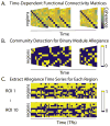
Schematic of Methods for Extracting Dynamic Module Time Series. (A) We represent the T (= 1190 (TRs) × 20 (subjects) × 4 (runs) = 95200) unique functional connectivity patterns as N × N adjacency matrices A. (B) Using community detection, we extract putative functional modules at each TR, and use a statistical comparison to a random null model to determine a region’s binary module allegiance. More specifically, we identify the community organization of ROIs and calculate the probability of ROI pairs’ congruent community allegiance for each time-point. The ROI pairs with higher than expected (via permutation tests) congruent community allegiance were thresholded to generate binarized pairwise allegiance matrices. (C) We reformat these data to separately store the allegiance time series of each ROI, which codes its co-allegiance with other ROIs to the same community (values of 1) as a function of time (TR).

Fig. 10

Schematic of Maximum Entropy Model of Brain Network Dynamics. (A) Accurate fitting of a MEM requires large amounts of data. We therefore combined data across all subjects before fitting a pairwise MEM to each ROI’s pattern of allegiance to functional modules. This fitting procedure produced an estimated interaction matrix for each ROI and each TR; colors indicate the strength of each element of the interaction matrix J_ij. (B) From the interaction matrices, we defined and characterized energy landscapes of the local community dynamics. Color indicates energy, with yellow indicating high energy and dark blue indicating low energy. Each minimum within each landscape is accompanied by an example network state, as defined by a binarized pattern of module allegiance (yellow indicating congruent module allegiance and dark blue indicating incongruent module allegiance) with other ROIs.

Fig. 11

Energy landscape of random ROIs time series. (A) Here we show (Left) the local minima, (Middle) the basin size of local minima states as the fraction of the number of basin states to the number of total possible states, and (Right) the Pearson correlation coefficient between any two ROIs’ vectors of basin size across minima states of the original time series. (B) Similar results are presented for the time series extracted from a random set of ROIs from ICA components.

References

1. Allen EA, Damaraju E, Plis SM, Erhardt EB, Eichele T, Calhoun VD. Tracking whole-brain connectivity dynamics in the resting state. Cereb Cortex. 2012;24:663–676. - PMC - PubMed
1. Andrews-Hanna JR, Smallwood J, Spreng RN. The default network and self-generated thought: component processes, dynamic control, and clinical relevance. Ann New Y Acad Sci. 2014;1316:29–52. - PMC - PubMed
1. Bassett DS, Porter MA, Wymbs NF, Grafton ST, Carlson JM, Mucha PJ. Robust detection of dynamic community structure in networks. ChaosL: an Interdisciplinary. J Nonlinear Sci. 2013a;23:013142. - PMC - PubMed
1. Bassett DS, Wymbs NF, Porter MA, Mucha PJ, Carlson JM, Grafton ST. Dynamic reconfiguration of human brain networks during learning. Proc Natl Acad Sci USA. 2011;108:7641–7646. - PMC - PubMed
1. Bassett DS, Wymbs NF, Rombach MP, Porter MA, Mucha PJ, Grafton ST. Task-based core-periphery organization of human brain dynamics. PLoS Comput Biol. 2013b;9:e1003171. - PMC - PubMed
Publication types
LinkOut - more resources