Invisible noise obscures visible signal in insect motion detection

Abstract

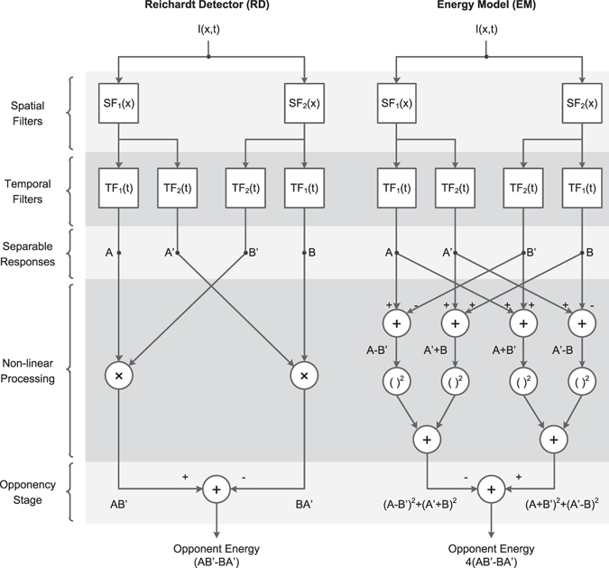
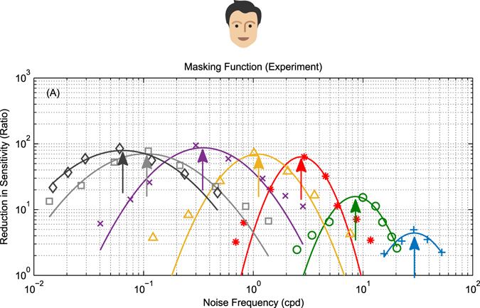
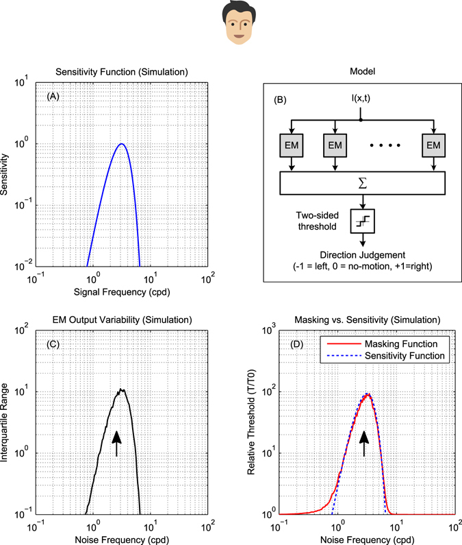
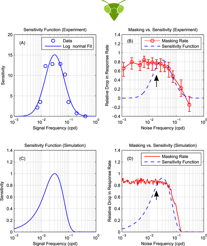
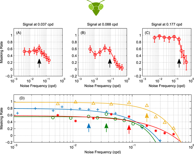
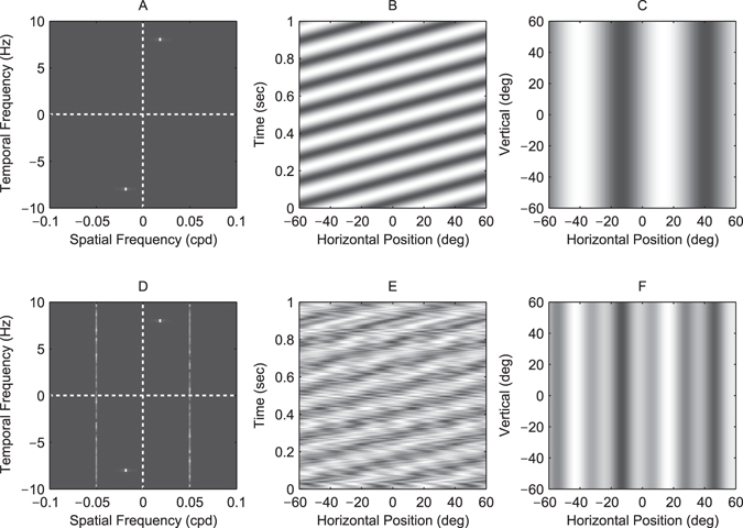
The motion energy model is the standard account of motion detection in animals from beetles to humans. Despite this common basis, we show here that a difference in the early stages of visual processing between mammals and insects leads this model to make radically different behavioural predictions. In insects, early filtering is spatially lowpass, which makes the surprising prediction that motion detection can be impaired by "invisible" noise, i.e. noise at a spatial frequency that elicits no response when presented on its own as a signal. We confirm this prediction using the optomotor response of praying mantis Sphodromantis lineola. This does not occur in mammals, where spatially bandpass early filtering means that linear systems techniques, such as deriving channel sensitivity from masking functions, remain approximately valid. Counter-intuitive effects such as masking by invisible noise may occur in neural circuits wherever a nonlinearity is followed by a difference operation.

Figure 1

Opponent energy models of motion detection. The Reichardt Detector (RD) and the Energy Model (EM) are two prominent opponent models in the literature of insect and mammalian motion detection. The two models are formally equivalent when the spatial and temporal filters are separable (as shown) and so their outputs and response properties are identical even though their structures are different. Both models use the outputs of several linear spatial and temporal filters (SF ₁, SF ₂, TF ₁ and TF ₂) to calculate two opponent terms and then subtract them to obtain a direction-sensitive measure of motion (opponent energy). Nonlinear processing is a fundamental ingredient of calculating motion energy and so both models include nonlinear operators before the opponency stage (multiplication in the RD and squaring in the EM). (Redrawn after Fig. 18 from ref. 8).

Figure 2

Spatiotemporal filter and opponent energy tuning in an opponent motion model. (A,B) Fourier spectra of rightward and leftward energies ((A + B′)² + (A′ − B)², Equation 6, and (A − B′)² + (A′ + B)², Equation 7) for example mammalian and insect opponent energy motion detectors (see Methods for details, Equations 18–22). The colored lines in each plot are 0.25 sensitivity contours. The Fourier spectra of leftward and rightward energies are very similar to the model’s filters in each case: spatially bandpass in mammals and low-pass in insects. (C,D) Opponent energy, AB′ − A′B, computed as the difference between rightward and leftward energies. In mammals, rightward and leftward responses do not overlap because the spatial filter are band-pass (panel A). In insects, the low-pass spatial filters cause an overlap between rightward and leftward responses (panel B) but this overlap is canceled at the opponency stage making opponent energy insensitive to low spatial frequencies (panel D).

Figure 3

Effect of noise on mammalian motion detectors. Measurements showing the effect of noise on motion detection sensitivity in humans (reproduced from Fig. 1b from ref. 5). The colored points show responses to different signal frequencies (marked by arrows); smooth curves represent masking functions drawn through the symbols by eye. Noise is most effective at masking the signal when its frequency is the same and less effective as its frequency changes in either direction.

Figure 4

For mammalian bandpass filters, the masking function reflects sensitivity. (A) Spatial sensitivity function of a mammalian band-pass energy-model motion detector, i.e., its response to single drifting gratings as a function of the grating spatial frequency. (B) Direction discrimination model based on an array of opponent models with the spatial tuning plotted in panel A. Opponent model outputs are pooled and passed through a two-sided threshold of value T to produce a ternary judgment of motion direction per stimulus presentation. (C) The variability of opponent model outputs across 500 simulated presentations (per noise frequency point) of a noisy stimulus consisting of a signal grating of 3 cpd and temporally-broadband noise. Signal frequency is marked on the plot with an arrow. Signal and noise had $\sqrt{2}$ and $20\sqrt{2}$ RMS contrast respectively. Adding noise did not change the mean of opponent output but had a significant effect on its spread. Output variance was highest when noise frequency was 3 cpd and lower as noise frequency changed in either direction, closely resembling the shape of the opponent model’s sensitivity function. (D) The masking function (red) was calculated based on these simulated results as T(f _n)/T ₀ where T(f _n) is the threshold corresponding to a 90% detection rate at each noise frequency and T ₀ is the detection threshold of an unmasked grating. The sensitivity function from (A) is reproduced, scaled, for comparison (blue dotted line). The masking function is a good approximation to the sensitivity.

Figure 5

For mantis motion detection, masking function does not reflect sensitivity. (A) The spatial sensitivity of mantis motion detectors at 8 Hz, measured using the same experimental paradigm, showing bandpass sensitivity in the range 0.01 to 0.1 cpd (reproduction of Fig. 3a in ref. 31). (B) Measurements showing the effect of noise on the detection of a moving grating in the praying mantis. Circles are masking rate M defined as M = (R ₀ − R)/R ₀ where R is the response rate (proportion of trials in which mantids responded optomotorally in the same direction as the signal grating) and R ₀ is the baseline (no-noise) response rate. Error bars are 95% confidence intervals calculated using simple binomial statistics. Signal frequency (0.0185 cpd) is marked on the plot with an arrow. The response rate measured at 0.03 cpd was slightly below baseline and so the calculated masking rate was negative. (C) Normalized sensitivity function of a motion energy model tuned to 0.03 cpd. (D) Simulated masking function (red) with the simulated sensitivity function reproduced for comparison (blue dotted line, scaled to same peak). Masking and sensitivity functions in the mantis are qualitatively different: noise below the lower end of the sensitivity function (~0.01 cpd) continues to mask the signal.

Figure 6

Mantis masking rate measurements at different signal frequencies. (A–C) Measurements of masking rate versus noise frequency in the mantis (for signal frequencies 0.037, 0.088 and 0.177 cpd) showing the same masking trends as Figure 5A (signal frequency 0.0185 cpd): noise continues to mask the signal significantly even if its frequency is below the spatial sensitivity passband of mantis motion detectors (~0.01 to 0.1 cpd). Circles are masking rate M defined as M = (R ₀ − R)/R ₀ where R is the response rate (proportion of trials in which mantids responded optomotorally in the same direction as the signal grating) and R ₀ is the baseline (no-noise) response rate. Error bars are 95% confidence intervals calculated using simple binomial statistics. Signal frequency is marked on each plot by an arrow. (D) Masking rate fits for the four signal frequencies combined, demonstrating a masking effect that is qualitatively different from humans (cf. Figure 3). Fitted functions are in the form $M(f)=a-\exp (b.\log (x)-c)$. Arrows indicate signal frequencies. Data-points are replotted from panels (A–C) and from Figure 5B.

Figure 7

Masked grating visual stimuli used in the experiment. (A,D) Spatiotemporal Fourier spectra, (B,E) space-time plots and (C,F) still frames of the visual stimulus in two conditions of the experiment. Panels (A–C) represent a no-noise condition: the stimulus is a moving grating at 0.0185 cpd and 8 Hz with no added noise. Panels (D–F) represent a masked condition: the stimulus consists of the same signal grating but with non-coherent temporally-broadband noise added at 0.05 cpd. There were in total 44 conditions in the experiment (4 unmasked and 40 masked gratings). Noise was always temporally broadband and its spatial frequency varied across conditions (in the range 0.0012 to 0.5 cpd).

References

1. Campbell FW, Robson J. Application of Fourier analysis to the visibility of gratings. Journal of Physiology. 1968;197:551. doi: 10.1113/jphysiol.1968.sp008574. - DOI - PMC - PubMed
1. Carandini M. What simple and complex cells compute. The Journal of Physiology. 2006;577:463–466. doi: 10.1113/jphysiol.2006.118976. - DOI - PMC - PubMed
1. Burge J, Geisler WS. Optimal disparity estimation in natural stereo images. Journal of Vision. 2014;14:1–1. doi: 10.1167/14.2.1. - DOI - PMC - PubMed
1. Batista J, Araújo H, et al. Stereoscopic depth perception using a model based on the primary visual cortex. PLoS One. 2013;8:e80745. doi: 10.1371/journal.pone.0080745. - DOI - PMC - PubMed
1. Anderson SJ, Burr DC. Spatial and temporal selectivity of the human motion detection system. Vision Research. 1985;25:1147–1154. doi: 10.1016/0042-6989(85)90104-X. - DOI - PubMed
Publication types
LinkOut - more resources