Violation of the virial theorem and generalized equipartition theorem for logarithmic oscillators serving as a thermostat

Abstract

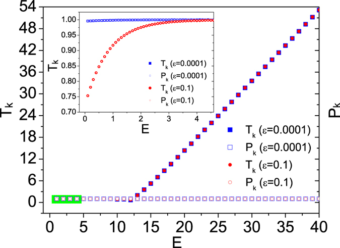
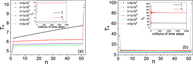
A logarithmic oscillator has been proposed to serve as a thermostat recently since it has a peculiar property of infinite heat capacity according to the virial theorem. In order to examine its feasibility in numerical simulations, a modified logarithmic potential has been applied in previous studies to eliminate the singularity at the origin. The role played by the modification has been elucidated in the present study. We argue that the virial theorem is practically violated in finite-time simulations of the modified log-oscillator illustrated by a linear dependence of kinetic temperature on energy. Furthermore, as far as a thermalized log-oscillator is concerned, our calculation based on the canonical ensemble average shows that the generalized equipartition theorem is broken if the temperature is higher than a critical temperature. Finally, we show that log-oscillators fail to serve as thermostats for their incapability of maintaining a nonequilibrium steady state even though their energy is appropriately assigned.

Figure 1

Kinetic temperature T _k and the quantity P _k as a function of the total energy E of the isolated log-oscillator for different ε. In our simulation, τ = 1, relaxation time and average time are 10⁸ and 2 × 10⁹ time steps, respectively. Numerical fitting gives T _k = 2(E − E _c) for the linearly increasing part. Inset: Enlarged view of low-energy part within the green rectangle.

Figure 2

Kinetic temperature T _k as a function of the total energy E of the isolated log-oscillator for different average time. Here τ = 1 and ε = 0.0001. The relaxation time is 10⁸ time steps for all three cases.

Figure 3

T _k as a function of the average time for an isolated oscillator with the total energy (a) E = 5 and (b) E = 25. The average is along two typical trajectories (see text for details) denoted by the blue line and the red line, respectively. The prediction by the virial theorem (T _k = P _k) is drawn by green lines as a reference. Here τ = 1, ε = 0.0001, the relaxation time is given by 10⁸ time steps. Note that the time unit of the right plot is billions (10⁹) of time steps. For such a long-time simulations, the energy drift in our simulations is controlled in the order of 10⁻⁴ (trajectory 1) and 10⁻⁷ (trajectory 2).

Figure 4

K _μ and P _μ as function of the evolution time for different Langevin thermostat’s temperature T. For a given time, K _μ and P _μ are calculated by ensemble average. Here τ = 1, ε = 0.0001, γ = 0.7, and the number of ensembles is 1 × 10⁶.

Figure 5

K _μ, P _μ as function of the scaled temperature T/τ. Here 10⁶ ensembles are used and each ensemble of the system evolves 10⁶ time steps. Here we set τ = 1, ε = 0.0001, and γ = 0.7.

Figure 6

Temperature profiles for different average time. Energy of respective log-oscillators is initially given by (a) E ₋ = 1 and E ₊ = 20; (b) E ₋ = 40 and E ₊ = 80. From top to bottom, the average time is 5 × 10⁵, 10⁶, 10⁸, 10⁹, 2 × 10⁹ and 5 × 10⁹ time steps, respectively. Inset: Temperatures of the left and right log-oscillators (denoted by T ₋ and T ₊) as a function of the average time. The parameters for log-oscillators are set by τ ₋ = 5, τ ₊ = 10 and ε = 0.0001. The coupling parameters between thermostats and the system are set by γ ₋ = 0.0005, γ ₊ = 0.00005. The system size N = 52.

References

1. Coffey, W. T. & Kalmykov, Y. P. The Langevin Equation: With Applications to Stochastic Problems in Physics, Chemistry and Electrical Engineering, vol. 27 (World Scientific, 2012).
1. Hoover, W. G. & Hoover, C. G. Time Reversibility, Computer Simulation, Algorithms, Chaos, vol. 13 of Advanced Series in Nonlinear Dynamics (World Scientific, 2012).
1. Campisi M, Zhan F, Talkner P, Hänggi P. Logarithmic oscillators: ideal hamiltonian thermostats. Phys. Rev. Lett. 2012;108:250601. doi: 10.1103/PhysRevLett.108.250601. - DOI - PubMed
1. Tuckerman, M. Statistical Mechanics: Theory and Molecular Simulation (Oxford University Press, 2010).
1. Campisi M, Hänggi P. Thermostated hamiltonian dynamics with log oscillators. J. Phys. Chem. B. 2013;117:12829–12835. doi: 10.1021/jp4020417. - DOI - PubMed
Publication types
LinkOut - more resources