Identifying populations sensitive to environmental chemicals by simulating toxicokinetic variability

Abstract

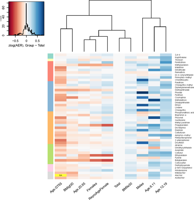
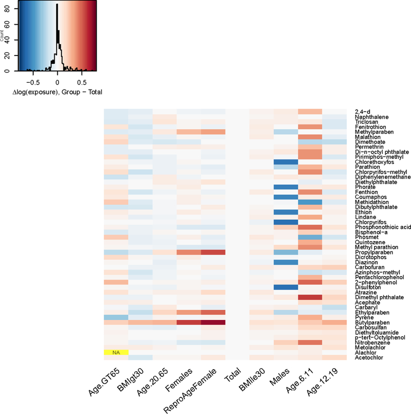
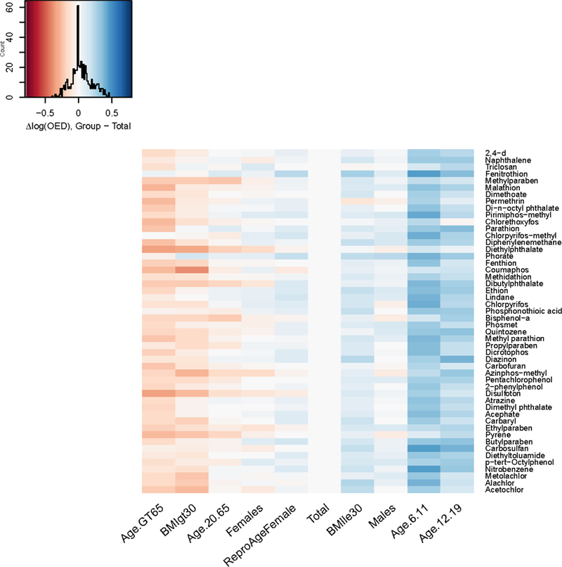
The thousands of chemicals present in the environment (USGAO, 2013) must be triaged to identify priority chemicals for human health risk research. Most chemicals have little of the toxicokinetic (TK) data that are necessary for relating exposures to tissue concentrations that are believed to be toxic. Ongoing efforts have collected limited, in vitro TK data for a few hundred chemicals. These data have been combined with biomonitoring data to estimate an approximate margin between potential hazard and exposure. The most "at risk" 95th percentile of adults have been identified from simulated populations that are generated either using standard "average" adult human parameters or very specific cohorts such as Northern Europeans. To better reflect the modern U.S. population, we developed a population simulation using physiologies based on distributions of demographic and anthropometric quantities from the most recent U.S. Centers for Disease Control and Prevention National Health and Nutrition Examination Survey (NHANES) data. This allowed incorporation of inter-individual variability, including variability across relevant demographic subgroups. Variability was analyzed with a Monte Carlo approach that accounted for the correlation structure in physiological parameters. To identify portions of the U.S. population that are more at risk for specific chemicals, physiologic variability was incorporated within an open-source high-throughput (HT) TK modeling framework. We prioritized 50 chemicals based on estimates of both potential hazard and exposure. Potential hazard was estimated from in vitro HT screening assays (i.e., the Tox21 and ToxCast programs). Bioactive in vitro concentrations were extrapolated to doses that produce equivalent concentrations in body tissues using a reverse dosimetry approach in which generic TK models are parameterized with: 1) chemical-specific parameters derived from in vitro measurements and predicted from chemical structure; and 2) with physiological parameters for a virtual population. For risk-based prioritization of chemicals, predicted bioactive equivalent doses were compared to demographic-specific inferences of exposure rates that were based on NHANES urinary analyte biomonitoring data. The inclusion of NHANES-derived inter-individual variability decreased predicted bioactive equivalent doses by 12% on average for the total population when compared to previous methods. However, for some combinations of chemical and demographic groups the margin was reduced by as much as three quarters. This TK modeling framework allows targeted risk prioritization of chemicals for demographic groups of interest, including potentially sensitive life stages and subpopulations.

Keywords: Environmental chemicals; High throughput; IVIVE; Risk assessment; Toxicokinetics.

Figure 1.

Plot matrix of pairwise density estimates of the parameters generated by HTTK-Pop, for a simulated population Ages 20–65 (N=1000). Solid lines represent data generated using the direct-resampling method; dotted lines represent data generated using the virtual-individuals method. Plot diagonal shows estimated one-dimensional marginal densities. Lower triangular portion of plot shows estimated contours of two-dimensional marginal densities for each pair of parameters. Deviations from concentric circles indicate correlation and/or departure from normal distribution.

Figure 2.

Median C_ss predicted using a generated population of N=1000 non-obese 20–50-year-olds, plotted against median C_ss derived from clearance values measured in vivo for 95 chemicals. Solid line: identity line. Dashed line: best-fit line to the full data set (log₁₀-transformed) (adjusted R²=0.3; intercept 0.16±0.08; slope 0.56±0.09). Dotted line: best-fit line to the log₁₀-transformed data set excluding the two chemicals with the highest literature-derived median C_ss (PFOS and PFOA) (adjusted R² = 0.22; intercept 0.2±0.09; slope 0.67±0.13). Shaded regions around each line denote the 99% confidence intervals around each fit.

Figure 3.

Comparisons of C_ss variability predicted using HTTK-Pop generated study populations averaged over 20 trials to in vivo C_ss variability (data collected in Johnson et al. 2006 [left panel] and Howgate et al. 2006 [right panel]). Each ellipse corresponds to a different in vivo study or pool of studies; each color corresponds to a chemical. For some chemicals, the results of multiple in vivo studies are included (represented by multiple ellipses in the same color). Ellipse centers are located at the median value in each dimension; ellipse axes encompass 95% confidence intervals on the observations in each dimension. The dashed line is the identity line. Ellipses centered at points on the identity line would indicate that the model predicted the same median C_ss as was observed in vivo. Perfect circles would indicate that the model predicted the same amount of variability in C_ss as was observed in vivo. Horizontally-elongated ellipses indicate that the model predicted less variability in C_ss than was observed in vivo; vertically-elongated ellipses indicate that the model predicted more variability in C_ss than was observed in vivo.

Figure 4.

Black box-and-whisker plots show the range of oral equivalent doses over a range of ToxCast AC₅₀ percentiles, for the 95^th percentile C_ss in the Total population. Black bars indicate oral equivalent dose corresponding the median AC₅₀. Boxes range from 25^th percentile AC₅₀ to 75^th percentile AC₅₀ equivalent doses. Whiskers range from 10^th percentile AC₅₀ to 90^th percentile AC₅₀ equivalent doses. Filled circles indicate 5^th and 95^th percentile AC₅₀ equivalent doses. Orange box plots show the range of the 95% confidence interval on median exposures inferred from NHANES biomonitoring data: bars indicate the median exposure. The distance between the lower black whisker (corresponding to the 10^th percentile AC₅₀ equivalent dose) and the upper edge of the orange box, on a log scale, is the AER. (Note: For reasons of space, O-ethyl o-(p-nitrophenyl) phenylphosphonothioate is denoted by the shorter name Phosphonothioic acid, and 4-(1,1,3,3-tetramethylbutyl)phenol is denoted by the shorter name p-tert-Octylphenol.)

Figure 5.

Difference in log₁₀ AER (number of orders of magnitude difference) between each demographic subgroup and the Total population. Chemicals are arranged from top to bottom in the same order as in Figure 4 (increasing AER for total population). Color bar at left indicates order of magnitude of AER in the Total population (from top to bottom: <=1, 100, 1 000, 10 000, etc.; no AERs on the order of 10 were observed in the Total population). The color of each cell represents the difference in log₁₀ AER from the Total population for the corresponding chemical (see color map with histogram, at top left). Red indicates lower AER (OED and exposure closer together); blue indicates higher AER (OED and exposure farther apart). (For reasons of space, O-ethyl o-(p-nitrophenyl) phenylphosphonothioate is denoted by the shorter name Phosphonothioic acid, and 4-(1,1,3,3-tetramethylbutyl)phenol is denoted by the shorter name p-tert-Octylphenol.)

Figure 6.

Difference in log₁₀ upper 95% confidence limit on median exposure between each demographic subgroup and the total population, for each chemical in the NHANES biomonitoring inference data set. Note that chemicals are arranged from top to bottom in the same order as Figure 6 (increasing AER).

Figure 7.

Difference in log₁₀ OED between each demographic subgroup and the total population, for each chemical in the NHANES biomonitoring inference data set. Note that chemicals are arranged from top to bottom in the same order as in Figure 6 (increasing AER).

References

1. Abdo N; Xia M; Brown CC; Kosyk O; Huang R; Sakamuru S, et al. Population-based in vitro hazard and concentration-response assessment of chemicals: the 1000 Genomes high-throughput screening Study. Environmental Health Perspectives 2015;123:458. - PMC - PubMed
1. Aylward LL; Hays SM Consideration of dosimetry in evaluation of ToxCast™ data. Journal of Applied Toxicology 2011;31:741–751 - PubMed
1. Barter ZE; Bayliss MK; Beaune PH; Boobis AR; Carlile DJ; Edwards RJ, et al. Scaling factors for the extrapolation of in vivo metabolic drug clearance from in vitro data: reaching a consensus on values of human micro-somal protein and hepatocellularity per gram of liver. Current Drug Metabolism 2007;8:33–45 - PubMed
1. Barter ZE; Chowdry JE; Harlow JR; Snawder JE; Lipscomb JC; Rostami-Hodjegan A Covariation of human microsomal protein per gram of liver with age: absence of influence of operator and sample storage may justify interlaboratory data pooling. Drug Metabolism and Disposition 2008;36:2405–2409 - PubMed
1. Baxter‐Jones AD; Faulkner RA; Forwood MR; Mirwald RL; Bailey DA Bone Mineral Accrual from 8 to 30 Years of Age: An Estimation of Peak Bone Mass. Journal of Bone and Mineral Research 2011;26:1729–1739 - PubMed
Substances
LinkOut - more resources