Haralick texture features from apparent diffusion coefficient (ADC) MRI images depend on imaging and pre-processing parameters

Abstract

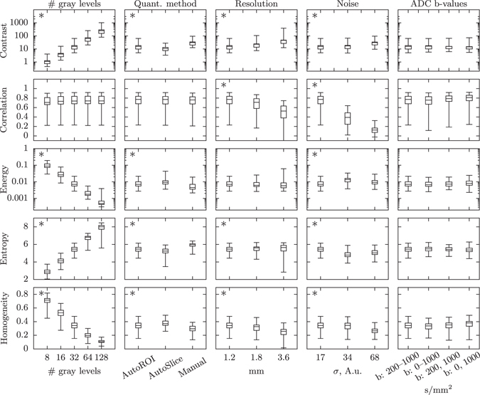
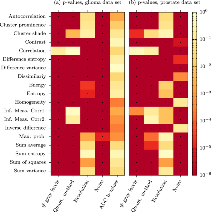
In recent years, texture analysis of medical images has become increasingly popular in studies investigating diagnosis, classification and treatment response assessment of cancerous disease. Despite numerous applications in oncology and medical imaging in general, there is no consensus regarding texture analysis workflow, or reporting of parameter settings crucial for replication of results. The aim of this study was to assess how sensitive Haralick texture features of apparent diffusion coefficient (ADC) MR images are to changes in five parameters related to image acquisition and pre-processing: noise, resolution, how the ADC map is constructed, the choice of quantization method, and the number of gray levels in the quantized image. We found that noise, resolution, choice of quantization method and the number of gray levels in the quantized images had a significant influence on most texture features, and that the effect size varied between different features. Different methods for constructing the ADC maps did not have an impact on any texture feature. Based on our results, we recommend using images with similar resolutions and noise levels, using one quantization method, and the same number of gray levels in all quantized images, to make meaningful comparisons of texture feature results between different subjects.

Figure 1

Changes in texture feature distributions with different imaging and pre-processing settings. The box plots show the distribution of contrast, correlation, energy, entropy and homogeneity for the 72 ROIs in the glioma data set. The box shows the first and third quartiles, with the median value indicated by the center line. The whiskers show the extreme values. An asterisk in the upper left corner indicates that at least one pair of settings is significantly different.

Figure 2

Probabilities that texture features are unaffected by changes in imaging or pre-processing steps. Heatmaps showing the probability (p-value) that all settings for a given parameter give the same texture feature values. The dots represent significant changes at the α = 0.01 level, with Bonferroni corrections. (a) Shows the result from the glioma data set, (b) from the prostate cancer data set.

Figure 3

The effect of ROI uncertainties to the texture features. The delineated glioma in a slice near the left lateral ventricle in a 73 year old male, from which the variations in the texture features were calculated in Table 1. The colormap shows the ADC map, fused on the T1-weighted contrast enhanced MPRAGE. An expansion or a shift by one voxel can include CSF in the ROI, which will increase the minimum and maximum values in the ROI, and will have an effect on the resulting texture features. The manual quantization method is less sensitive to this shift.

Figure 4

A description of how Haralick’s texture features are calculated. In an example 4 × 4 image ROI, three gray levels are represented by numerical values from 1 to 3. The GLCM is constructed by considering the relation of each voxel with its neighborhood. In this example we only look at the neighbor to the right. The GLCM acts like a counter for every combination of gray level pairs in the image. For each voxel, its value and the neighboring voxel value are counted in a specific GLCM element. The value of the reference voxel determines the column of the GLCM and the neighbor value determines the row. In this ROI, there are two instances when a reference voxel of 3 “co-occurs” with a neighbor voxel of 2, indicated in solid blue, and there is one instance of a reference voxel of 3 with a neighbor voxel of 1, indicated in dashed red. The normalized GLCM represents the frequency or probability of each combination to occur in the image. The Haralick texture features are functions of the normalized GLCM, where different aspects of the gray level distribution in the ROI are represented. For example, diagonal elements in the GLCM represent voxels pairs with equal gray levels. The texture feature “contrast” gives elements with similar gray level values a low weight but elements with dissimilar gray levels a high weight. It is common to add GLCMs from opposite neighbors (e.g. left-right or up-down) prior to normalization. This generates symmetric GLCMs, since each voxel has been the neighbor and the reference in both directions. The GLCMs and texture features then reflect the “horizontal” or “vertical” properties of the image. If all neighbors are considered when constructing the GLCM, the texture features are direction invariant.

Figure 5

The effect of using different minimum and maximum values when quantizing the image. The images show how different minimum and maximum values influence the result when quantizing the original image, prior to constructing the GLCM. (a) Shows the original image with 4096 gray levels. In (b) the image has been quantized to 8 gray levels, and the minimum and maximum gray levels have been set to that of the ROI, dashed outline. In (c), the image has been quantized to 8 gray levels and minimum and maximum gray levels have been set based on the entire image. There are large regions of uniform gray levels in (c), the texture is very different compared to (b), and the only difference is how the maximum and minimum gray levels were chosen.

Figure 6

The span of ADC values in the data sets. Boxplots of ADC minimum and maximum values as well as the range of ADC values within each tumor for the glioma data set and the prostate cancer data set respectively.

References

1. Haralick RM, Shanmugam K, Dinstein I. Textural Features for Image Classification. IEEE Transactions on Systems, Man, and Cybernetics. 1973;3:610–621. doi: 10.1109/TSMC.1973.4309314. - DOI
1. Materka A. Texture analysis methodologies for magnetic resonance imaging. Dialogues in clinical neuroscience. 2004;6:243–250. - PMC - PubMed
1. Lerski R, et al. Computer analysis of ultrasonic signals in diffuse liver disease. Ultrasound in Medicine & Biology. 1979;5:341–343. doi: 10.1016/0301-5629(79)90004-8. - DOI - PubMed
1. Skorton DJ, Collins SM, Woskoff SD, Bean Ja, Melton HE. Range- and azimuth-dependent variability of image texture in two- dimensional echocardiograms. Circulation. 1983;68:834–840. doi: 10.1161/01.CIR.68.4.834. - DOI - PubMed
1. O’Connor JPB, et al. Imaging intratumor heterogeneity: Role in therapy response, resistance, and clinical outcome. Clinical Cancer Research. 2015;21:249–257. doi: 10.1158/1078-0432.CCR-14-0990. - DOI - PMC - PubMed