Low-dimensional spike rate models derived from networks of adaptive integrate-and-fire neurons: Comparison and implementation

Abstract

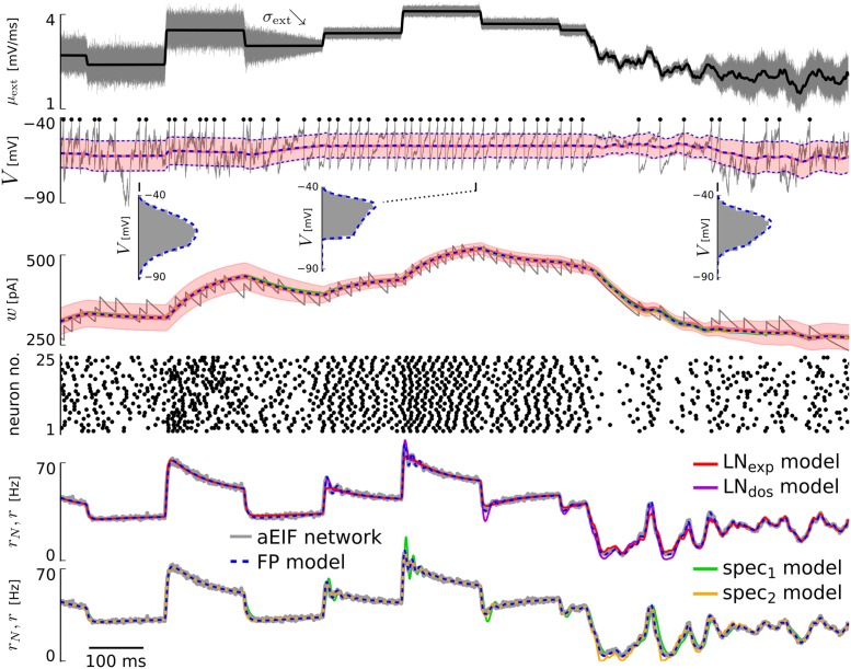
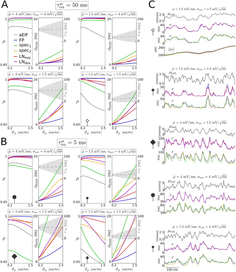
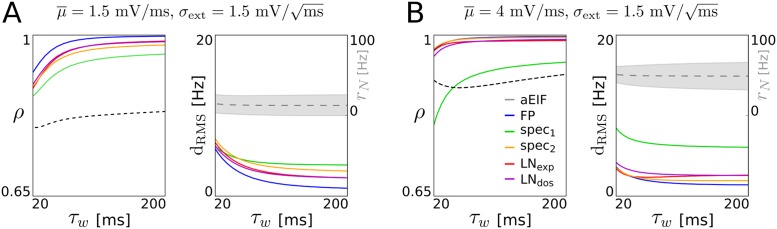
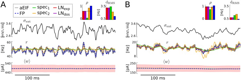
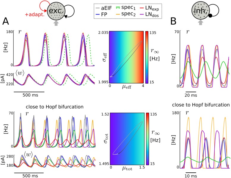
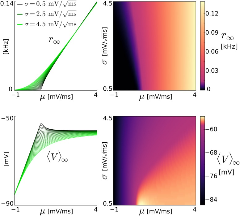
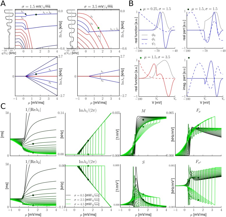
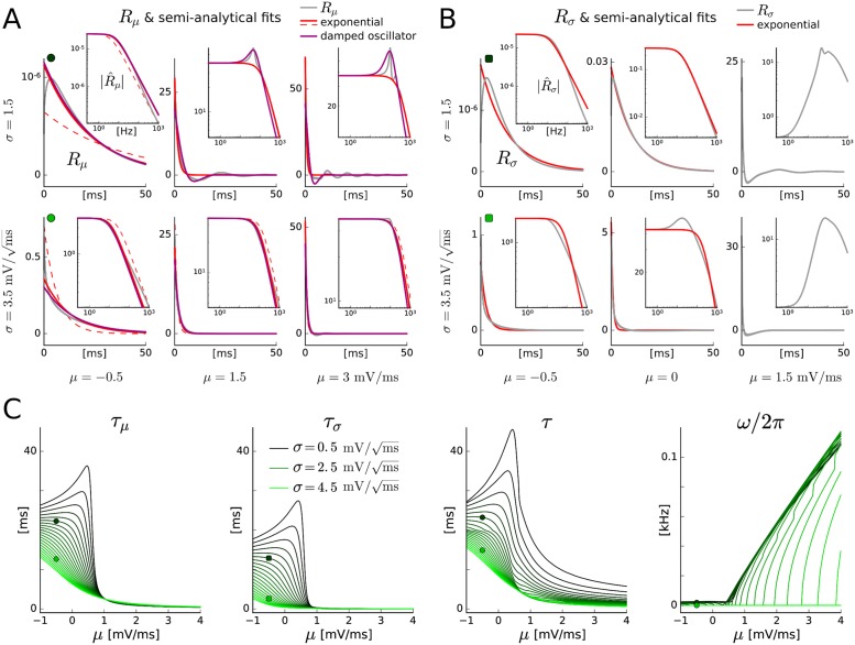
The spiking activity of single neurons can be well described by a nonlinear integrate-and-fire model that includes somatic adaptation. When exposed to fluctuating inputs sparsely coupled populations of these model neurons exhibit stochastic collective dynamics that can be effectively characterized using the Fokker-Planck equation. This approach, however, leads to a model with an infinite-dimensional state space and non-standard boundary conditions. Here we derive from that description four simple models for the spike rate dynamics in terms of low-dimensional ordinary differential equations using two different reduction techniques: one uses the spectral decomposition of the Fokker-Planck operator, the other is based on a cascade of two linear filters and a nonlinearity, which are determined from the Fokker-Planck equation and semi-analytically approximated. We evaluate the reduced models for a wide range of biologically plausible input statistics and find that both approximation approaches lead to spike rate models that accurately reproduce the spiking behavior of the underlying adaptive integrate-and-fire population. Particularly the cascade-based models are overall most accurate and robust, especially in the sensitive region of rapidly changing input. For the mean-driven regime, when input fluctuations are not too strong and fast, however, the best performing model is based on the spectral decomposition. The low-dimensional models also well reproduce stable oscillatory spike rate dynamics that are generated either by recurrent synaptic excitation and neuronal adaptation or through delayed inhibitory synaptic feedback. The computational demands of the reduced models are very low but the implementation complexity differs between the different model variants. Therefore we have made available implementations that allow to numerically integrate the low-dimensional spike rate models as well as the Fokker-Planck partial differential equation in efficient ways for arbitrary model parametrizations as open source software. The derived spike rate descriptions retain a direct link to the properties of single neurons, allow for convenient mathematical analyses of network states, and are well suited for application in neural mass/mean-field based brain network models.

Fig 1. Example of aEIF network response and output of derived models for varying input.

From top to bottom: Mean input μ_ext (black) together with input standard deviation σ_ext (gray, visualized for one neuron by sampling the respective white noise process ξ_ext,i). 2^nd row: Membrane voltage V of one neuron (gray, with spike times highlighted by black dots) and membrane voltage statistics from the excitatory coupled aEIF population of 50,000 neurons (red) and from the FP model (blue dashed): mean ± standard deviation over time, as well as voltage histograms (gray) and probability densities p(V, t) (blue dashed) at three indicated time points. 3^rd row: Adaptation current w of one neuron (gray) and mean adaptation currents of all models ± standard deviation for the aEIF network (shaded area). Note that differences in the mean adaptation currents of the different models are hardly recognizable. 4^th row: Spike times of a subset of 25 neurons randomly chosen from the network. Below: Spike rate r of the LN cascade based models (LN_exp, LN_dos) and the spectral models (spec₁, spec₂) in comparison to the FP model and the aEIF network (r_N). The values of the coupling parameters were J = 0.05 mV, K = 100, τ_d = 3 ms.

Fig 2. Reproduction accuracy of the reduced models for variations of the mean input.

Pearson correlation coefficient (ρ) and root mean square distance (d_RMS) between the spike rate time series r_N(t) of the aEIF population and r(t) of each derived model (FP, spec₁, spec₂, LN_exp, LN_dos) for different strengths of baseline mean input $\overline{\mu }$, input standard deviation σ_ext, mean input variation ϑ_μ and for a large value of time constant ${\tau }_{\text{ou}}^{\mu }$ (A, moderately fast variations) as well as a smaller value (B, rapid variations). The input-output correlation (between μ_ext and r_N) is included as a reference (black dashed lines), and mean ± standard deviation of the population spike rate r_N are indicated (gray dashed lines, shaded areas). For each parametrization, activity time series of 60 s duration were generated (from 50,000 aEIF neurons and each derived model), from which the first second was omitted (each) to exclude transients, since the initial conditions of the models were not matched. Representative time series examples are shown on the right side with parameter values indicated (C), where empty and filled symbols correspond to large and small correlation time ${\tau }_{\text{ou}}^{\mu }$, respectively, relating the examples to the panels A and B. The adaptation current traces were excluded in all but the first example to allow for a larger number of parameter points.

Fig 3. Effect of adaptation current timescale on reproduction accuracy.

Performance measures and population spike rate statistics (cf. Fig 2A and 2B) as a function of the adaptation time constant τ_w, that takes values between 20 ms (equal to the membrane time constant) and 200 ms (used throughout the rest of the study). The spike-triggered adaptation increment b was co-varied (antiproportional to τ_w) such that the product τ_w b = 8 pAs is fixed for all shown parametrizations. The input mean μ_ext(t) fluctuates with timescale ${\tau }_{\text{ou}}^{\mu }=50\text{ms}$ and strength ϑ_μ = 0.54 mV/ms (same value as for examples in Fig 2C) around a smaller (A) and a larger (B) baseline mean $\overline{\mu }$, while the input deviation σ_ext is constant. Note that the rightmost parametrization of A corresponds to Fig 2C (top example) and is contained in Fig 2A (bottom right) while that of B is shown in Fig 2A (bottom left).

Fig 4. Performance for variations of the input variance.

Time series of population spike rate and mean adaptation current from the different models in response to varying ${\sigma }_{\text{ext}}^2$ for large mean input and rapid variations, μ_ext = 4 mV/ms, ${\tau }_{\text{ou}}^{{\sigma }^2}=5\text{ms}$ (A) and for small mean input and moderately fast variations, μ_ext = 1.5 mV/ms, ${\tau }_{\text{ou}}^{{\sigma }^2}=50\text{ms}$ (B). The values for the remaining input parameters were ${\overline{\sigma }}_{\text{ext}}^2=9{\text{mV}}^2/\text{ms}$, ϑ_σ² = 2 mV²/ms. For the aEIF population 〈w〉± standard deviation are visualized (red shaded areas). Note that the mean adaptation time series of all models as well as the spike rates of the cascade based models are on top of each other. The indicated Pearson correlation coefficients (with dashed input-output correlation) and root mean square distances were calculated from simulated spike rate time series of 60 s duration from which the first second was excluded, as the initial conditions of the models were not matched. In A the correlation ρ (but not the distance d_RMS) between the spike rates of the model spec₁ and the aEIF population) is strongly decreased due to a small time lag between the two time series which is difficult to see in the figure.

Fig 5. Network-generated oscillations.

Oscillatory population spike rate and mean adaptation current of 50,000 excitatory coupled aEIF neurons and each of the derived models (for constant external input moments) generated by the interplay of recurrent excitation/adaptation current (A) and by delayed recurrent inhibition (B). In addition, the limit cycle of the LN_exp model is shown in terms of the (quantity) steady-state spike rate r_∞ as a function of effective input moments μ_eff, ${\sigma }_{\text{eff}}^2$ (A, top) and for the spec₂ model in dependence of the total input moments (μ_tot, ${\sigma }_{\text{tot}}^2$ (A, bottom). The phase of the cycle is visualized by grayscale color code (increasing phase from black to white). The values for the input, adaptation and coupling parameters were μ_ext = 1.5 mV/ms, ${\sigma }_{\text{ext}}=2\text{mV}/\sqrt{\text{ms}}$, a = 3 nS, b = 30 pA (A, top), μ_ext = 1.275 mV/ms, ${\sigma }_{\text{ext}}=1.5\text{mV}/\sqrt{\text{ms}}$, a = 3 nS, b = 60 pA (A, bottom), K = 1000, J = 0.03 mV, τ_d = 3 ms (A, both). In B adaptation was removed (a = b = 0) and delays were identical d_ij = d; input and coupling parameter values were μ_ext = 1.5 mV/ms, ${\sigma }_{\text{ext}}=1.5\text{mV}/\sqrt{\text{ms}}$, K = 1000, J = −0.0357 mV, d = 10 ms (top) and μ_ext = 3 mV/ms, ${\sigma }_{\text{ext}}=2\text{mV}/\sqrt{\text{ms}}$, K = 1000, J = −0.087 mV, d = 5 ms (bottom).

Fig 6. Steady-state spike rate and mean membrane voltage for a population of EIF neurons.

r_∞ and 〈V〉_∞ for an uncoupled population of EIF neurons (aEIF with a = b = 0) as a function of (generic) input mean μ and standard deviation σ, calculated from the (steady-state) Fokker-Planck equation, shown in two different representations (left and right, each).

Fig 7. Spectrum of the Fokker-Planck operator L and related quantities.

A: regular eigenvalues of $\mathcal{L}$ (blue) and diffusive ones (red) with real and imaginary part (top and bottom, respectively) as a function of the mean input μ for small noise intensity σ (left) and larger input fluctuations (right). The first two dominant eigenvalues λ₁, λ₂ are indicated together with discontinuities in the real (λ₂) and imaginary part (λ₁ and λ₂), respectively. The stationary eigenvalue λ₀ = 0 is shown in gray. Note that the value of the mean input μ at which the eigenvalue λ_n changes from real to complex values depends on the noise amplitude σ and the eigenvalue index n which is difficult to see in the figure. The narrow winding curves attached to the left side of the respective spectra represent the lower bound flux q(V_lb) for μ_min = −1.5 mV/ms as a function of (real) eigenvalue candidate λ. The flux axis has a logarithmic scale between the large ticks (absolute values between 10⁻¹⁰ and 10⁻² kHz) and is linear around the dashed zero value. The open circles denote the eigenvalues, i.e., those λ that satisfy q(V_lb) = 0. Note that q(V_lb) ranges over several orders of magnitude. B: stationary eigenfunction ϕ₀ = p_∞ (gray) and nonstationary eigenfunctions ϕ₁ of $\mathcal{L}$ and ψ₁ of ${\mathcal{L}}^{*}$ corresponding to the first dominant eigenvalue λ₁ for three different input parameter values indicated by the triangle and circles in A (same units of μ and σ as therein). The eigenfunctions are biorthonormalized, but (only) for visualization truncated at V = −100 mV and furthermore individually scaled to absolutely range within the unit interval of arbitrary units [a.u.]. C: first and second dominant eigenvalues λ₁, λ₂ with real and imaginary part (that are also indicated in A), as well as additional (real-valued) quantities of the model spec₂ (M, S, F_μ, F_σ²) as a function of input mean μ and noise strength σ in steps of $0.2\text{mV}/\sqrt{\text{ms}}$ from small values (black) to larger ones (green). The dots indicate identical parameter values to the spectra of A and the eigenfunctions of B (darker: $\sigma =1.5\text{mV}/\sqrt{\text{ms}}$, brighter green: $\sigma =3.5\text{mV}/\sqrt{\text{ms}}$).

Fig 8. Linear rate response functions and quantities for the cascade models.

Linear rate response functions of EIF neurons subject to white noise input for modulations of the input mean around μ with constant σ: R_μ(t; μ, σ) in kHz/V (A, gray) and for modulations of the input standard deviation around σ with constant μ: R_σ(t; μ, σ) in $\text{kHz}/(\text{V}·\sqrt{\text{ms}}$) (B, gray). These functions are calculated in the Fourier domain for a range of modulation frequencies [${\widehat{R}}_{\mu }(f;\mu ,\sigma )$ in 1/V and ${\widehat{R}}_{\sigma }(f;\mu ,\sigma )$ in $1/(\text{V}·\sqrt{\text{ms}}$)] (insets, gray; absolute values are shown), and fit using an exponential function exploiting asymptotic results for ${\widehat{R}}_{\mu }$ (A, red dashed), as well as considering a range of frequencies (A and B, red solid). In addition, ${\widehat{R}}_{\mu }$ is fit using a damped oscillator function (A, violet). The details of the fitting procedures are described in the text. C: quantities (τ_μ, τ_σ, τ and ω) from the linear filter approximations (cf. A, B), required for the LN_exp and LN_dos model variants (Eqs (85), (87) and (89)), as a function of μ and σ.

References

1. Shadlen MN, Newsome WT. The variable discharge of cortical neurons: implications for connectivity, computation, and information coding. J Neurosci. 1998; 18(10):3870–3896. - PMC - PubMed
1. Gerstner W, Kistler WM, Naud R, Paninski L. Neuronal dynamics: from single neurons to networks and models of cognition. Cambridge University Press; 2014.
1. Harris KD, Shepherd GMG. The neocortical circuit: themes and variations. Nat Neurosci. 2015; 18(2):170–181. 10.1038/nn.3917 - DOI - PMC - PubMed
1. Okun M, Steinmetz NA, Cossell L, Iacaruso MF, Ko H, Barthó P, et al. Diverse coupling of neurons to populations in sensory cortex. Nature. 2015; 521(7553):511–515. 10.1038/nature14273 - DOI - PMC - PubMed
1. Brette R, Gerstner W. Adaptive exponential integrate-and-fire model as an effective description of neuronal activity. J Neurophysiol. 2005; 94(5):3637–3642. 10.1152/jn.00686.2005 - DOI - PubMed
LinkOut - more resources