Autoreject: Automated artifact rejection for MEG and EEG data

Abstract

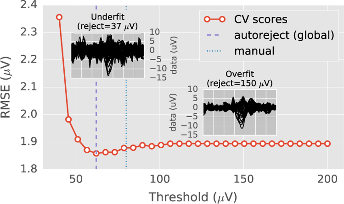
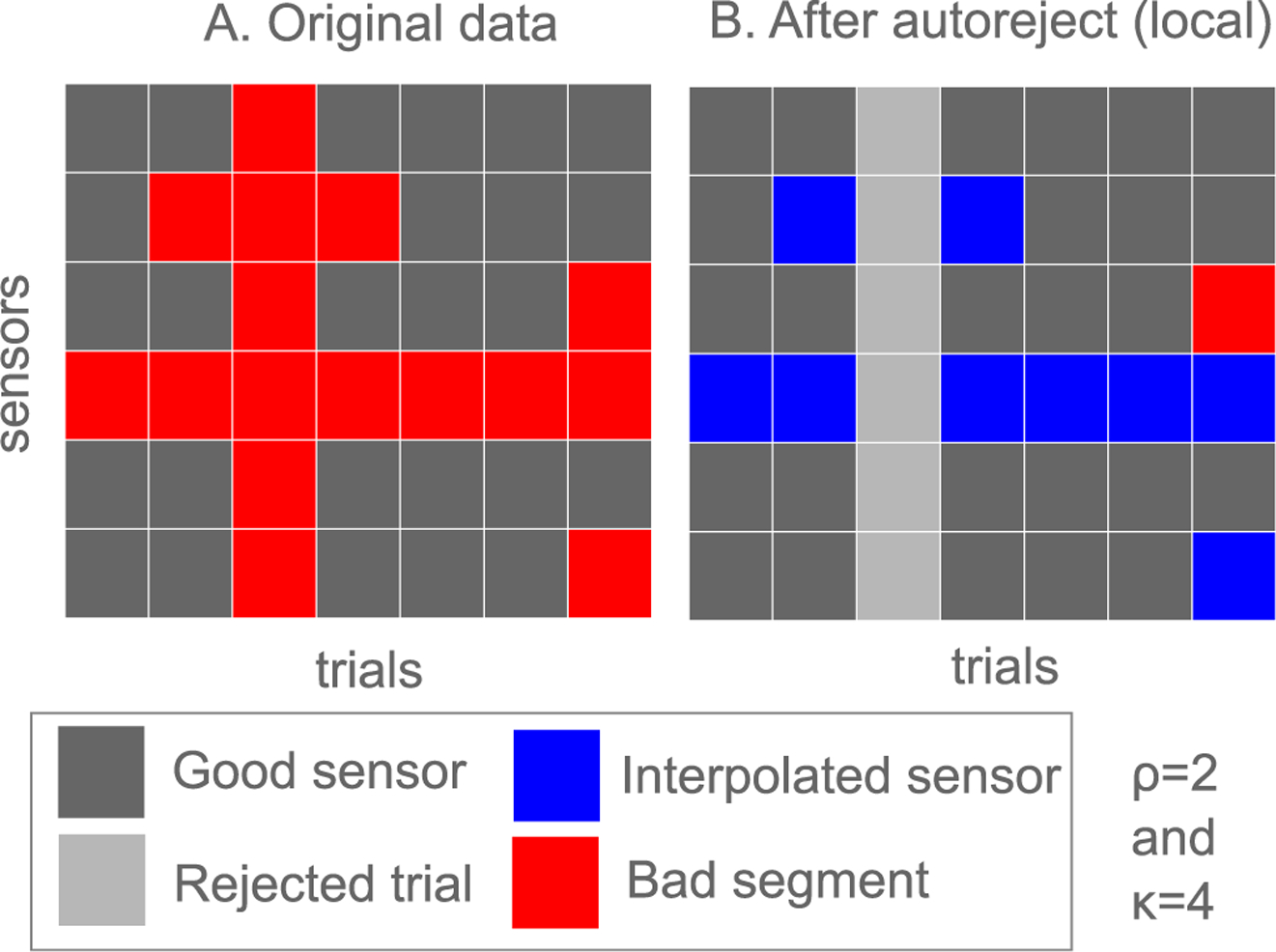
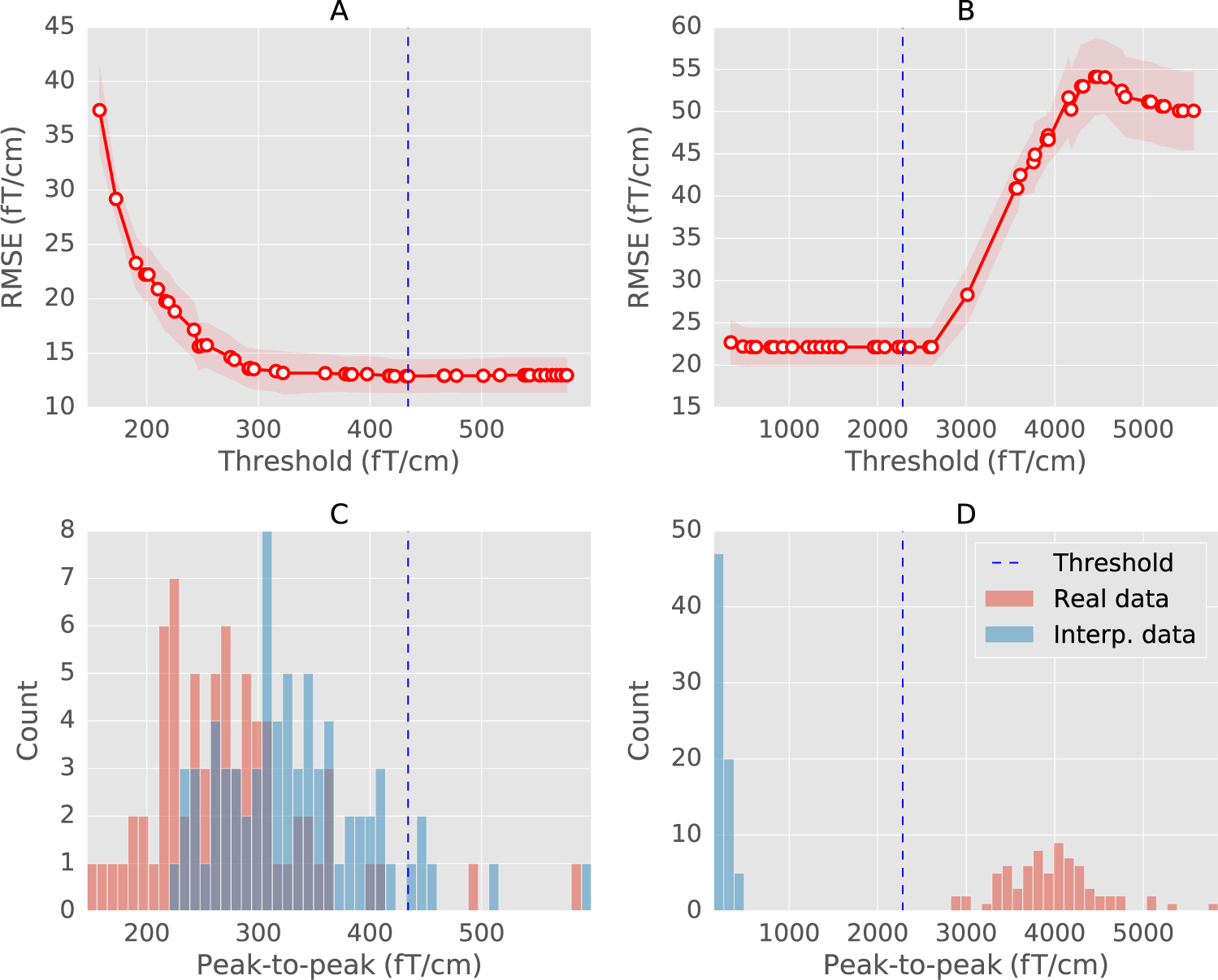
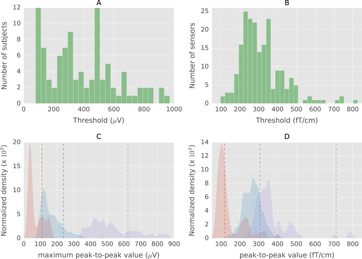
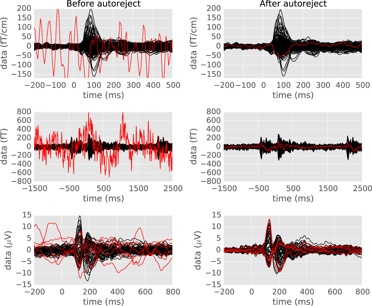
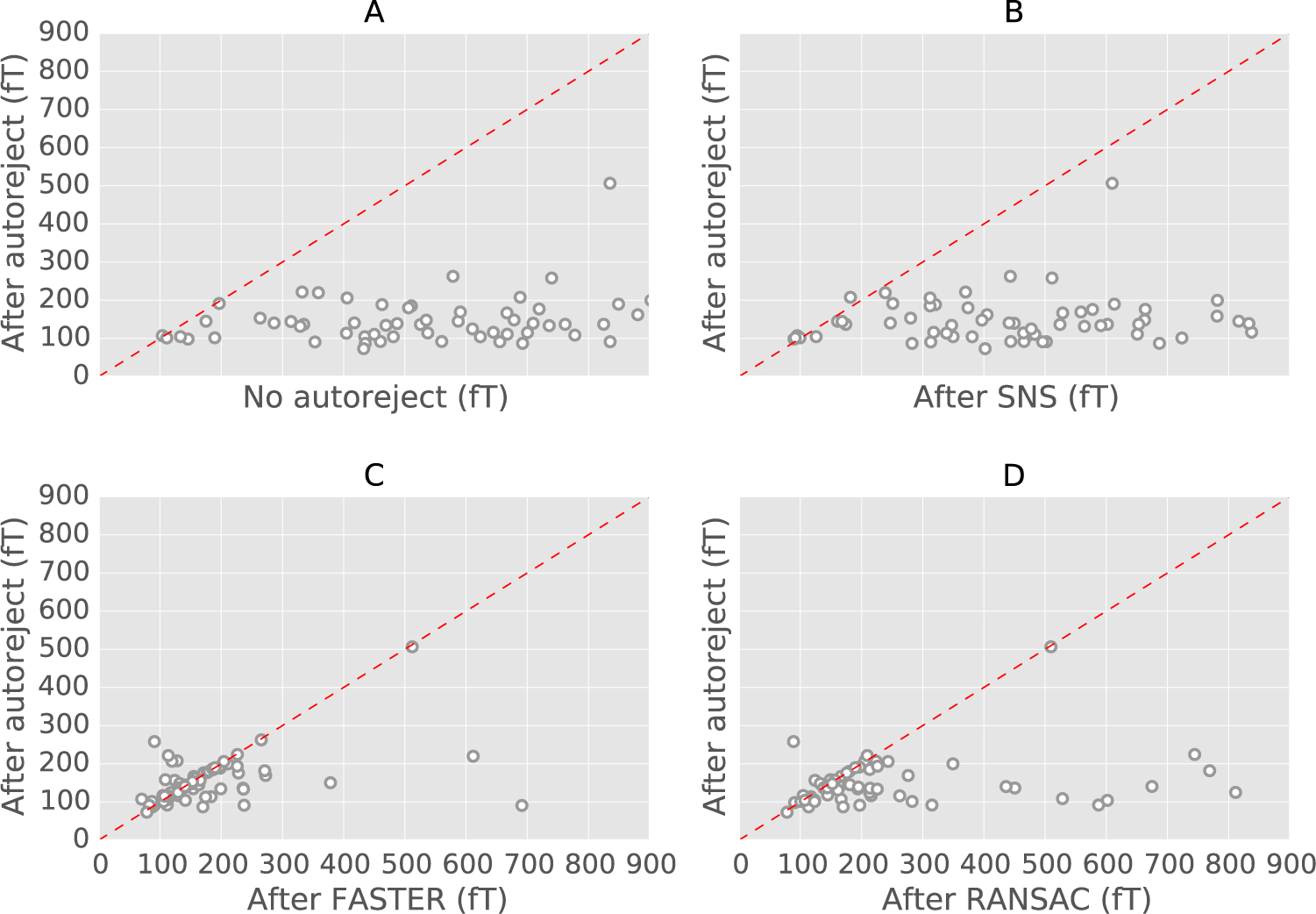
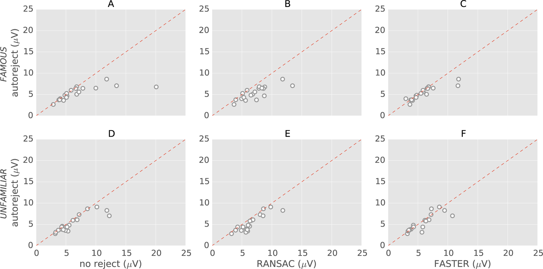
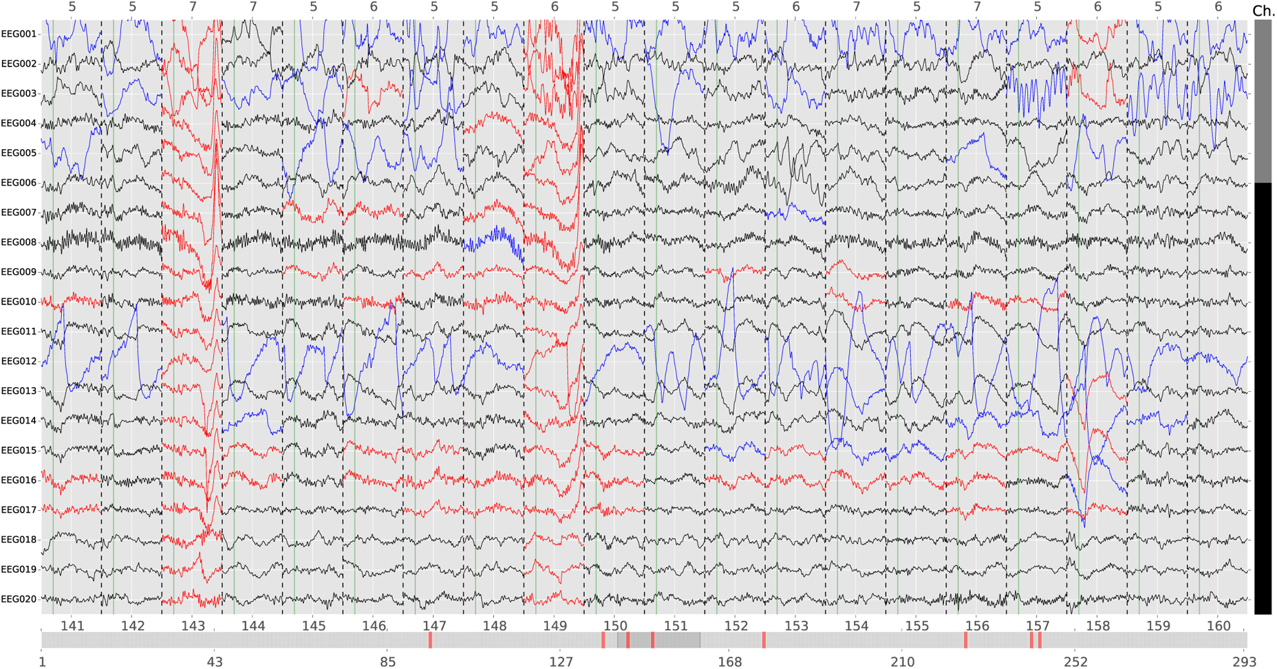
We present an automated algorithm for unified rejection and repair of bad trials in magnetoencephalography (MEG) and electroencephalography (EEG) signals. Our method capitalizes on cross-validation in conjunction with a robust evaluation metric to estimate the optimal peak-to-peak threshold - a quantity commonly used for identifying bad trials in M/EEG. This approach is then extended to a more sophisticated algorithm which estimates this threshold for each sensor yielding trial-wise bad sensors. Depending on the number of bad sensors, the trial is then repaired by interpolation or by excluding it from subsequent analysis. All steps of the algorithm are fully automated thus lending itself to the name Autoreject. In order to assess the practical significance of the algorithm, we conducted extensive validation and comparisons with state-of-the-art methods on four public datasets containing MEG and EEG recordings from more than 200 subjects. The comparisons include purely qualitative efforts as well as quantitatively benchmarking against human supervised and semi-automated preprocessing pipelines. The algorithm allowed us to automate the preprocessing of MEG data from the Human Connectome Project (HCP) going up to the computation of the evoked responses. The automated nature of our method minimizes the burden of human inspection, hence supporting scalability and reliability demanded by data analysis in modern neuroscience.

Keywords: Automated analysis; Cross-validation; Electroencephalogram (EEG); Human Connectome Project (HCP); Magnetoencephalography (MEG); Preprocessing; Statistical learning.

Fig. 1.

Cross-validation error as a function of peak-to-peak rejection threshold on one EEG dataset. The root mean squared error (RMSE) between the mean of the training set (after removing the trials marked as bad) and the median of the validation set was used as the cross-validation metric (Autoreject (global)). The two insets show the average of the trials as “butterfly plots” (each curve representing one sensor) for very low and high thresholds. For low thresholds, the RMSE is high because most of the trials are rejected (underfit). At high thresholds, the model does not drop any trials (overfit). The optimal data-driven threshold (autoreject, global) with minimum RMSE is somewhere in between. It closely matches the human threshold.

Fig. 2.

A schematic diagram explaining how autoreject (local) works. (A) Each cell here is an element of the indicator matrix C_ij described in the section on Autoreject (local). Sensor-level thresholds are found and bad segments are marked for each sensor. Bad segments shown in red are where C_ij =1 (B) Trials are rejected if the number of bad sensors is greater than κ and otherwise, the worst ρ sensors are interpolated.

Fig. 3.

(A) and (B) The cross-validation curve obtained with sequential Bayesian optimization (see section on Bayesian optimization for an explanation) for a regular (MEG 2523) and a globally bad sensor (MEG 2443) from the MNE sample dataset. The mean RMSE is shown in red circles with error bounds in red shades. The red shaded region shows the lower and upper bounds between which the optimization is carried out. Vertical dashed line marks the estimated threshold. (C) and (D) Histogram of peak-to-peak amplitudes of trials in the sensor. The histograms are computed separately for the real data (red) and the data interpolated from other sensors (blue). The estimated threshold correctly marks all the trials as bad for the globally bad sensor.

Fig. 4.

A. Histogram of thresholds for subjects in the EEGBCI dataset with autoreject (global) B. Histogram of sensor-specific thresholds in gradiometers for the MNE sample dataset (see Results). C. Normalized kernel density plots of maximum peak-to-peak value across sensors for three subjects in the EEGBCI data. Vertical dashed lines indicate estimated thresholds. Density plots and thresholds corresponding to the same subject are the same color. D. Normalized Kernel Density plots of peak-to-peak values for three MEG sensors in the MNE sample dataset. The threshold indeed has to be different depending on the data (subject and sensor).

Fig. 5.

The evoked response (average of data across trials) on three different datasets before and after applying autoreject — the MNE sample data, the HCP data and the EEG faces data. Each sensor is a line on the plots. On the left, manually annotated bad sensors are shown in red. The algorithm finds the bad sensors automatically and repairs them for the relevant trials. Note that it can even fix multiple sensors at a time and works for different modalities of data acquisition.

Fig. 6.

Scatter plots for the results with the HCP data. For each method, the ‖·‖_∞ norm of the difference between the HCP ground truth and the method is taken. Each circle is a subject. (A) autoreject (local) against no rejection, (B) autoreject (local) against Sensor Noise Suppression (SNS) (SNS), (C) autoreject against FASTER, (D) autoreject (local) against RANSAC. Data points below the dotted red line indicate subjects for which autoreject (local) outperforms the alternative method.

Fig. 7.

Scatter plots for the results with the 19 subjects from Faces dataset. The plots in the first row: (A), (B) and (C) are for the condition “famous”, whereas the plots in the second row: (D), (E) and (F) are for the condition “unfamiliar” faces. For each method, the ‖·‖_∞ norm of the difference between the ground truth and the estimates is computed. Each circle is a subject. Data points below the dotted red line indicate subjects for which autoreject (local) outperforms the alternative method.

Fig. 8.

An example diagnostic plot from an interactive viewer with autoreject (local). The data plotted here is subject 16 for the condition ‘famous’ in the EEG faces data. Each row is a different sensor. The trials are concatenated along the x axis with dotted vertical lines separating consecutive trials. Each trial is numbered at the bottom and its corresponding trigger code is at the top. The horizontal scroll bar at the bottom allows browsing trials and the vertical scroll bar on the right is for browsing sensors. A trial which is marked as bad is shown in red on the horizontal scroll bar and the corresponding column for the trial is also red. A data segment in a good trial is either i) Good (in black) ii) Bad and interpolated (blue), or iii) Bad but not interpolated (in red). Note that the worst sensors in a trial are typically interpolated.

References

1. Barachant A, Andreev A, Congedo M, 2013. The Riemannian Potato: an automatic and adaptive artifact detection method for online experiments using Riemannian geometry. in: TOBI Workshop lV, pp. 19–20.
1. Basirat A, Dehaene S, Dehaene-Lambertz G, 2014. A hierarchy of cortical responses to sequence violations in three-month-old infants. Cognition 132, 137–150. - PubMed
1. Bergstra JS, Bardenet R, Bengio Y, Kégl B, 2011. Algorithms for hyper-parameter optimization. in: Advances in Neural Information Processing Systems, pp. 2546–2554.
1. Bigdely-Shamlo N, Kreutz-Delgado K, Robbins K, Miyakoshi M, Westerfield M, Bel-Bahar T, Kothe C, Hsi J, Makeig S, 2015. Hierarchical event descriptor (HED) tags for analysis of event-related EEG studies. in: Global Conference on Signal and Information Processing (GlobalSIP), IEEE, pp. 1–4.
1. Bigdely-Shamlo N, Mullen T, Kothe C, Su K-M, Robbins K, 2015. The PREP pipeline: standardized preprocessing for large-scale EEG analysis. Front. Neuroinform 9. - PMC - PubMed
Publication types