. 2017 Jul 11;114(28):E5693-E5702.
doi: 10.1073/pnas.1704856114. Epub 2017 Jun 26.

Simulating tactile signals from the whole hand with millisecond precision

Affiliations

Simulating tactile signals from the whole hand with millisecond precision

Hannes P Saal et al. Proc Natl Acad Sci U S A. .

Abstract

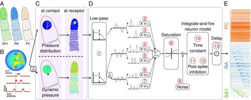
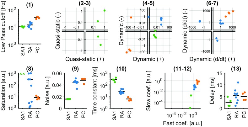
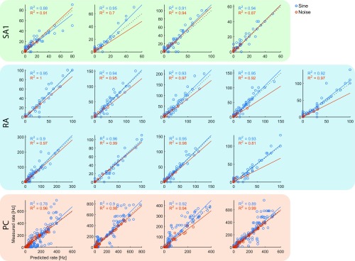
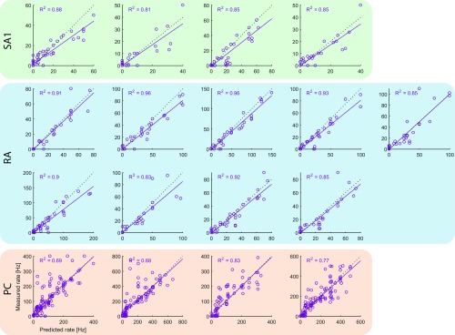
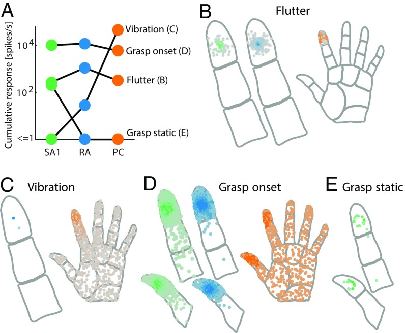
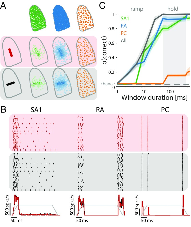
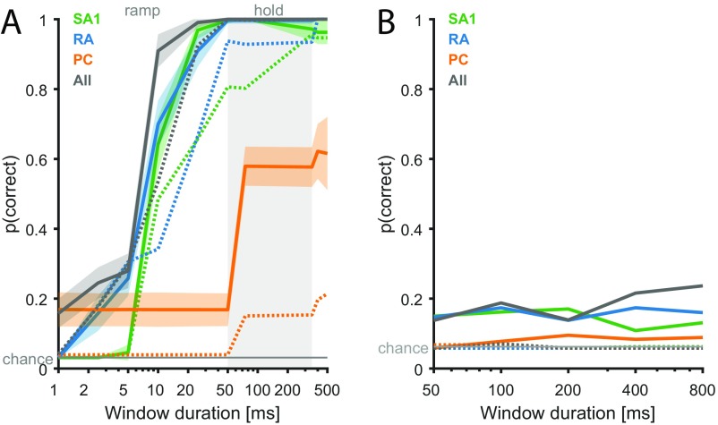
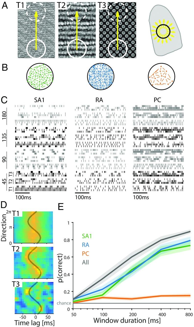
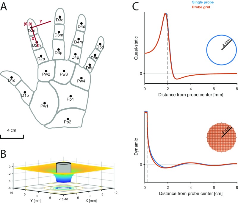
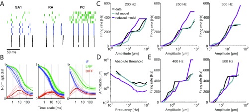
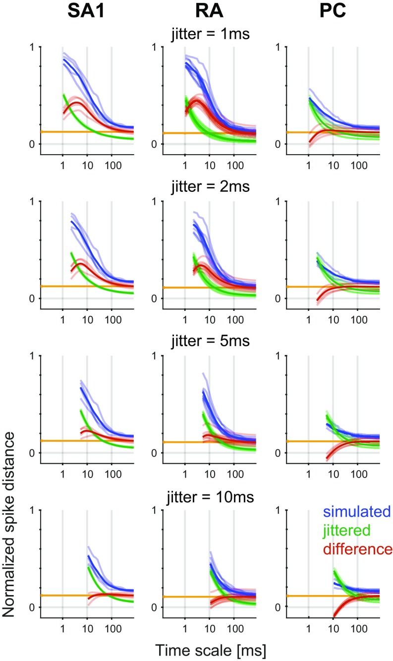
When we grasp and manipulate an object, populations of tactile nerve fibers become activated and convey information about the shape, size, and texture of the object and its motion across the skin. The response properties of tactile fibers have been extensively characterized in single-unit recordings, yielding important insights into how individual fibers encode tactile information. A recurring finding in this extensive body of work is that stimulus information is distributed over many fibers. However, our understanding of population-level representations remains primitive. To fill this gap, we have developed a model to simulate the responses of all tactile fibers innervating the glabrous skin of the hand to any spatiotemporal stimulus applied to the skin. The model first reconstructs the stresses experienced by mechanoreceptors when the skin is deformed and then simulates the spiking response that would be produced in the nerve fiber innervating that receptor. By simulating skin deformations across the palmar surface of the hand and tiling it with receptors at their known densities, we reconstruct the responses of entire populations of nerve fibers. We show that the simulated responses closely match their measured counterparts, down to the precise timing of the evoked spikes, across a wide variety of experimental conditions sampled from the literature. We then conduct three virtual experiments to illustrate how the simulation can provide powerful insights into population coding in touch. Finally, we discuss how the model provides a means to establish naturalistic artificial touch in bionic hands.

Keywords: computational model; mechanoreceptor; skin mechanics; somatosensory periphery; tactile afferent.


Conflict of interest statement

The authors declare no conflict of interest.

Figures

Fig. 1.
Fig. 1.
Overview of the model. (A) Receptors are distributed across the skin given the known innervation densities of SA1, RA, and PC afferents. (B) The stimulus—in this case, a vibrating embossed letter A scanned across the skin—is defined as the time-varying depth at which each small patch of skin (here dubbed a pin) is indented (with a spatial resolution of 0.1 mm). The traces in Lower show the time-varying depth at the three locations on the skin indicated by the red dots in Upper. (C) The mechanics model relies on two parts: (Upper) modeling the distribution of stresses using a quasistatic elastic model and (Lower) modeling dynamic pressure and surface wave propagation. Left shows the surface deformation of the skin, and Right shows the resulting pattern of stresses at the location of the receptors. (D) The spiking responses are determined by leaky IF models using different sets of up to 13 parameters (marked in red numbers) for individual SA1, RA, and PC afferents fit based on peripheral recordings to skin vibrations. Adapted from ref. . (E) The output of the model is the spike train of each afferent in the population. Raster of the response of the afferent population sampled as in A to the stimulus shown in B (only active afferents are included). Note that the SA1s (in contact) only encode the spatial aspect of the stimulus, that the PCs encode from the whole finger phase-lock with the 200-Hz vibration, and that the RAs show mixed spatial and vibration responses.
Fig. S1.
Fig. S1.
Parameters for individual afferent models by type. Values generally cluster by afferent type, reflecting the observed differences in response properties across afferent classes and similarities within class. (1) Low-pass filter cutoff frequency. (2 and 3) Weights for positive and negative components of quasistatic stress (set to zero for RA and PC). (4 and 5) Weights for positive and negative components of dynamic stress. (6 and 7) Weights for positive and negative components of dynamic stress derivative (set to zero for SA1). (8) Saturation parameter (no saturation for SA1). (9) Gaussian noise added to the membrane potential (resting potential is zero, and a spike is triggered at one). (10) Membrane potential time constant. (11 and 12) Weights for the fast and slow components of the postspike inhibitory kernels. (13) Delay parameter accounting for conduction velocity.
Fig. S2.
Fig. S2.
Measured vs. predicted firing rates for all fitted models on the training data (blue, sinusoidal; red, noise). Dotted lines denote unity, whereas solid lines denote best fits. Table S1 shows slopes, intercepts, and a breakdown of the total error.
Fig. S3.
Fig. S3.
Measured vs. predicted firing rates for all fitted models on the test data (diharmonic vibrations). Dotted lines denote unity, whereas solid lines denote best fits. Table S1 shows slopes, intercepts, and a breakdown of the total error.
Fig. 2.
Fig. 2.
Spike timing. (A) Vector strength for actual (black) and modeled (blue and orange) RA afferents at 40 Hz and PC afferents at 300 Hz. Horizontal lines denote averages. (B–D) Recorded (black tick marks) and simulated (colored) spike trains for example (B) SA1, (C) RA, and (D) PC afferents in response to a noise and a sinusoidal stimulus. (E) Normalized difference in the spike distance between modeled and jittered spike trains to measured spike trains for the three afferent classes as a function of jitter level. Shaded lines show means for individual afferent, and dark lines show means across afferents. Vertical black ticks indicate the points at which the models become significantly worse than the jittered data.
Fig. S4.
Fig. S4.
Additional response properties. (A and B) Examples of (Upper) phase advance and (Lower) entrainment plateaus exhibited by a (A) recorded and (B) simulated RA afferent at a vibratory frequency of 40 Hz. A was reproduced from ref. . (C) Responses of a recorded (75) and modeled SA1 afferent to ramp-and-hold indentations at different depths. (D) Responses of a recorded (26) and modeled RA afferent to different ramp speeds. For both C and D, Top shows the indentation depth of the probe over time, Middle shows actual responses of afferents recorded in humans, and Bottom shows the responses of simulated afferents. (E and F) Edge enhancement. Firing rates for (E) recorded and (F) simulated RA afferents as a function of their location with respect to bar stimuli (shown in gray). Recorded and simulated RA fibers exhibit little spatial modulation; overall firing rates are also lower than for SA1 afferents. E was reproduced from ref. . (G and H) RF size vs. indentation depth for (G) actual and (H) simulated afferents. Although RF sizes are relatively independent of indentation depth for SA1 fibers, those of RA fibers grow with increasing depth, a property also exhibited by simulated afferents. G was reproduced from ref. . (I and J) Minimum amplitude required to elicit a response as a function of distance from the RF hot spot for (I) actual and (J) modeled RA afferents. The minimum amplitude begins to rise sharply at about 1 mm distance in both actual and modeled afferents. I was reproduced from ref. . (KP) Mean population response strength for recorded (77) and simulated (K and L) SA1, (M and N) RA, and (O and P) PC afferents to sinusoidal stimulation at different amplitudes and frequencies. The darkest lines correspond to the highest amplitudes used (1 mm peak to peak), and every lighter shade corresponds to a decrease in amplitude by 6 dB, down to –36 dB.
Fig. 3.
Fig. 3.
Basic response properties of simulated afferents. (A) Measured responses of an SA1 afferent to ramp-and-hold indentations at different depths (from ref. 75) and simulated responses of an SA1 fiber to those same stimuli. (B) Measured responses of an RA afferent to ramps at different speeds (from ref. 26) and simulated responses of an RA fiber to the same stimuli. In A and B, Top shows the indentation depth of the probe over time, Middle shows actual responses of afferents recorded in humans, and Bottom shows the responses of simulated afferents. (C) RF sizes (black, median; error bars, 25th and 75th percentiles) measured for SA1, RA, and PC afferents (27). (D) RF sizes of simulated afferents when stimulated and estimated in the same way as in C. The models exhibit the property that RA fibers tend to have larger RFs than SA1 fibers and that PC fibers have by far the largest RFs. (E, G, and I) Measured absolute (black) and tuning (red) thresholds for (E) SA1, (G) RA, and (I) PC afferents at different frequencies (76). (F, H, and J) Modeled absolute (black) and tuning (red) thresholds, corresponding to data shown in E, G, and I.
Fig. 4.
Fig. 4.
Spatial representation. (A) Reconstruction of the SA1, RA, and PC signals for various letters scanned across the skin (4). (B–E) Surround suppression. Average firing rates for (B and D) recorded (34) and (C and E) simulated (B and C) SA1 and (D and E) RA afferents as a function of the number of probes that are contacting the skin. Both recorded and simulated SA1 afferents exhibit stronger surround suppression than their RA counterparts. (F and G) Edge enhancement. Firing rates for (F) recorded (33) and (G) simulated SA1 afferents as function of their location with respect to bar stimuli (shown in gray). Edges of bars evoke higher firing rates for both recorded and simulated afferents.
Fig. 5.
Fig. 5.
Population responses for different tactile experiences. (A) Total number of spikes per second across simulated SA1, RA, and PC populations for four different types of tactile stimuli, the response distributions of which are shown in B–E. Spike counts across different afferent populations and stimuli vary by several orders of magnitude. Generally, all afferent types respond to a given stimulus, but in rare cases, a whole afferent population might be silent. (B) Spatial distribution of afferent responses (green, SA1; blue, RA; orange, PC) to a flutter stimulus (15 Hz) applied to the D2 fingertip through a small circular probe. Movie S1 shows a representation of the response over time. (C) Spatial distribution of responses for a 300-Hz vibration. Note that PC afferents located all over the hand respond to this stimulus. (D) Spatial distribution of responses during the onset of a two-finger grasp executed with D1 and D2. The sudden contact and fast ramp up of the contact force cause PC afferents all over the hand to respond, whereas only SA1 and RA afferents close to the contact locations respond. (E) Spatial distribution of responses during the static (hold) period of a two-finger grasp. RA and PC afferents are silent, whereas the SA1 afferent directly at the contact location responds weakly. Movie S2 shows a representation of the grasp response over time.
Fig. 6.
Fig. 6.
Insights from population responses: decoding the orientation of an indented edge. (A, Upper) Sampled afferent populations (SA1 in green, RA in blue, and PC in orange). (A, Lower) Their response strengths to indented edges at 2 of 32 orientations tested (0° and 90°). Darker colors indicate higher firing rates. (B, Upper) Responses of 30 selected SA1 and RA fibers to edge indented at two different orientations depicted in red and black. (B, Lower) Peri-stimulus time histogram (PSTH) of the afferent population response for each type to the two orientations, with the temporal profile of the stimulus superimposed in gray. (C) Classification performance for each afferent type as well as the total population for different window durations using spike count. Lines are means, and shaded areas show the SDs; the dashed lines denote chance level.
Fig. S5.
Fig. S5.
Classification of edge orientation and motion direction. (A) Edge orientation classification accuracy (over 32 orientations) for each afferent type and different window durations using a 2-ms temporal resolution (q= 500). Dotted lines show the performance for q= 0 for comparison (as in Fig. 6C). Lines are means, and shaded areas show SDs over afferents. (B) Motion direction classification accuracy (over 16 directions) for each afferent type and different window durations using raw spike trains. Solid lines show performance based on spike count (q= 0), whereas dotted lines are based on a 2-ms temporal resolution (q= 500). Shaded areas show SD across afferents.
Fig. 7.
Fig. 7.
Insights from population responses: decoding the direction of textured surfaces scanned across the finger. (A, Left) Three textured surfaces were scanned along the direction indicated by the yellow arrow over a patch of fingertip (denoted by the circle superimposed on the fingertip in A, Right) in 16 directions (shown with arrows on the fingertip). (B) Location of sampled afferents over the contact area for each class. Segments between afferents show pairs selected to compute cross-correlations. (C) Responses of three example afferents to different textures (labeled T1–T3 in A) scanned in four directions (angles on the left are relative to distal direction). (D) Cross-correlogram of a selected RA pair in response to 16 different directions. The gray trace shows the expected peak in the cross-correlogram given a pair of identical neurons responding to a sinusoidal grating. The resulting trace is a cosine with amplitude that is determined by distance between the RFs divided by the stimulus speed and phase that depends on their relative orientation. (E) Performance of the direction classifier (across textures) using correlograms for each afferent type and different window durations. Solid lines denote means, and shaded areas are SEMs.
Fig. S6.
Fig. S6.
Skin mechanics model. (A) Schematic of the hand used in the model. The reference coordinate system is centered on the center of the index fingertip. Different hand regions are defined that determine the innervation densities of the different afferent types. (B) Skin deflection profile resulting from the indentation of a circular pin (shown in gray; radius =2 mm). (C, Upper) Quasistatic and (C, Lower) dynamic components resulting from a 200-Hz vibration exerted with a single pin (radius = 2 mm; blue trace) or a grid of evenly spaced pins (spacing = 0.1 mm; radius = 0.05 mm). Receptor depth was set to 0.5 mm.
Fig. S7.
Fig. S7.
Model validation. (A) Comparison of spike timing precision between the IF and LNP models. Shown are raster plots of spikes evoked in the three afferent classes by five repetitions of one of the diharmonic stimuli (Left, SA1; Center, RA; Right, PC). Both measured (black) and simulated spikes (IF in blue and LNP in green) are shown. (B) Normalized spike distance between measured and simulated spike trains as a function of timescale (1/q). IF actual distance is in blue; LNP actual distance is in green. Shaded lines show the average distance across all conditions in the diharmonic vibration dataset for each afferent model. Dark lines show averages across afferents. Red traces (DIFF) show the difference between predictions of the two models: the IF model is better than LNP at all timescales but especially at the timescales that have been shown to be most informative for the different afferent classes (10 ms for SA1, 5 ms for RA, and 1 ms for PC). (C–E) Reduced model fits. Removing or clamping IF model parameters during the fitting process leads to impaired accuracy in reproducing well-known afferents response properties as illustrated in C–E. (C) Missing entrainment plateaus for a PC model at three different frequencies when the model was refit without postspike inhibition (parameters 11 and 12). (D) Absolute thresholds that were roughly one-half an order of magnitude too low when a PC model was refit with the decay variable clamped. (E) Excessive firing rates when a PC model was fit without a saturation term.
Fig. S8.
Fig. S8.
Spike timing precision. Difference in normalized distance between simulated (blue) and jittered (green) spike trains to measured spike trains for three afferent classes as a function of temporal resolution. The pairwise difference between the two distances is shown in red. Each row corresponds to a different jitter SD value (1, 2, 5, and 10 ms). Shaded lines show means for individual afferents, and dark lines show means across afferents. The orange vertical lines correspond to the mean distance differences caused by difference in spike count. The red line being below the orange line indicates that the simulated responses are closer to the measured response than the jittered ones.

References

    1. Johansson RS, Vallbo AB. Tactile sensibility in the human hand: Relative and absolute densities of four types of mechanoreceptive units in glabrous skin. J Physiol. 1979;286:283–300. - PMC - PubMed
    1. Johansson RS, Flanagan JR. Coding and use of tactile signals from the fingertips in object manipulation tasks. Nat Rev Neurosci. 2009;10:345–359. - PubMed
    1. Saal HP, Bensmaia SJ. Touch is a team effort: Interplay of submodalities in cutaneous sensibility. Trends Neurosci. 2014;37:689–697. - PubMed
    1. Phillips JR, Johnson KO, Hsiao SS. Spatial pattern representation and transformation in monkey somatosensory cortex. Proc Natl Acad Sci USA. 1988;85:1317–1321. - PMC - PubMed
    1. Manfredi LR, et al. The effect of surface wave propagation on neural responses to vibration in primate glabrous skin. PLoS One. 2012;7:e31203. - PMC - PubMed

Publication types

LinkOut - more resources