Distinct Correlation Structure Supporting a Rate-Code for Sound Localization in the Owl's Auditory Forebrain

Abstract

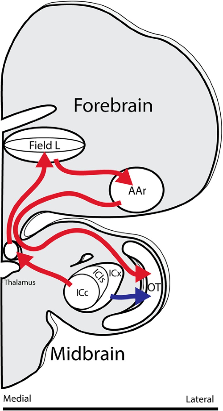
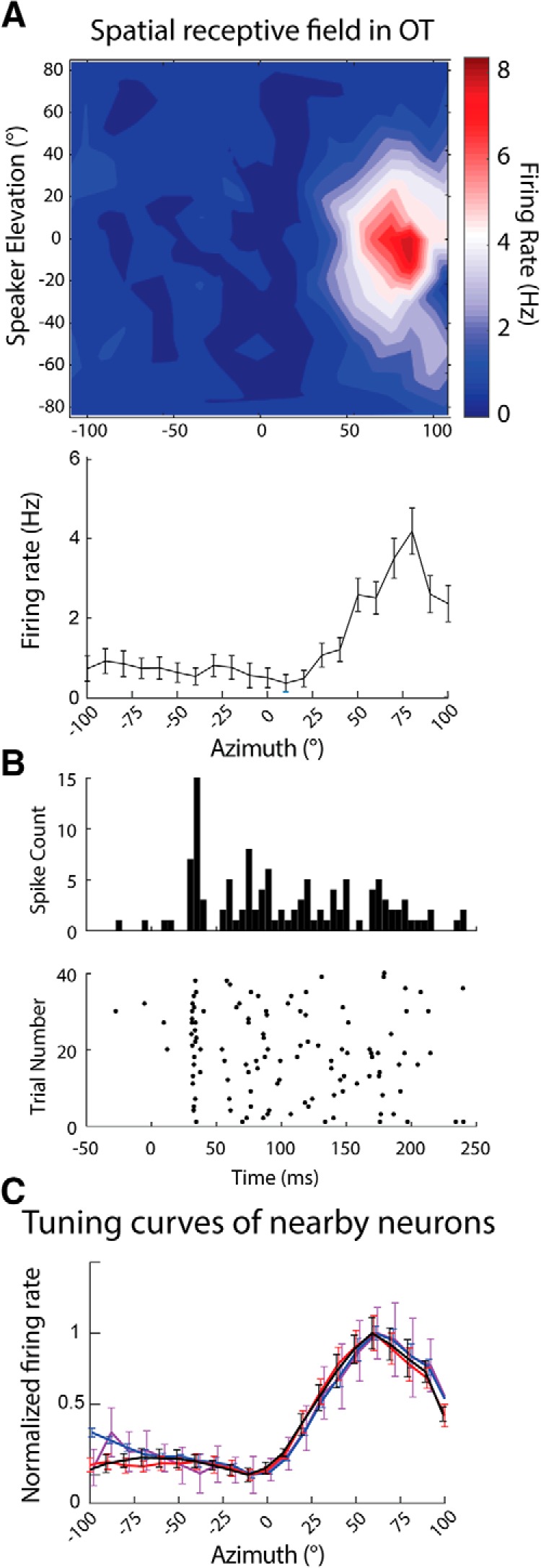
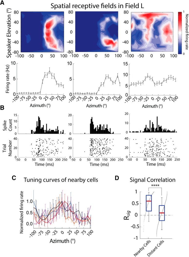
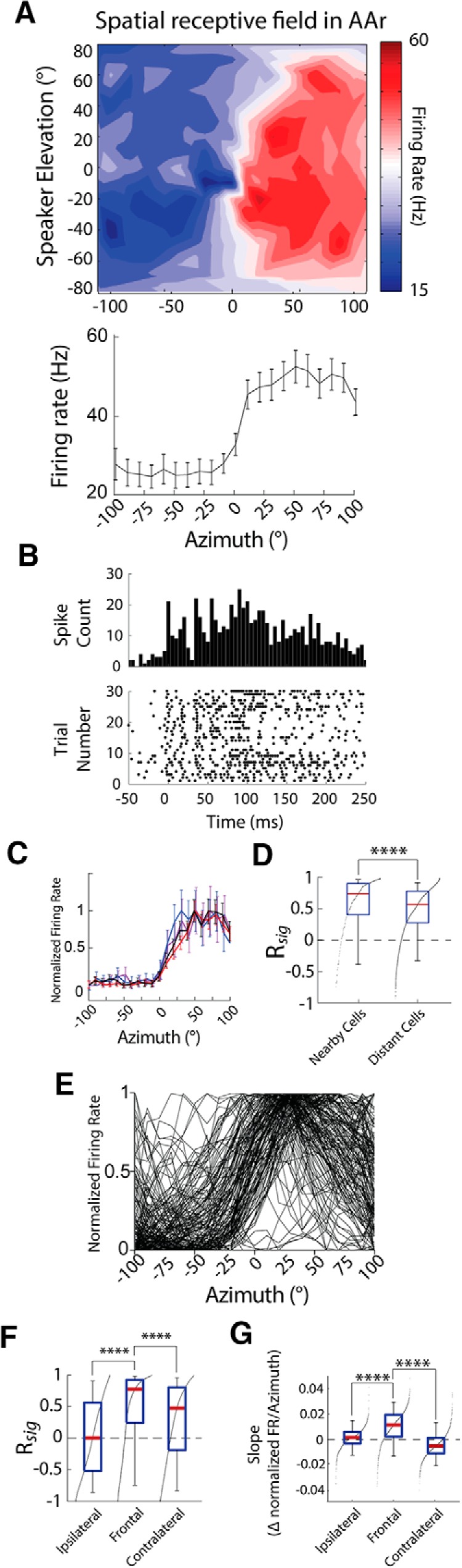
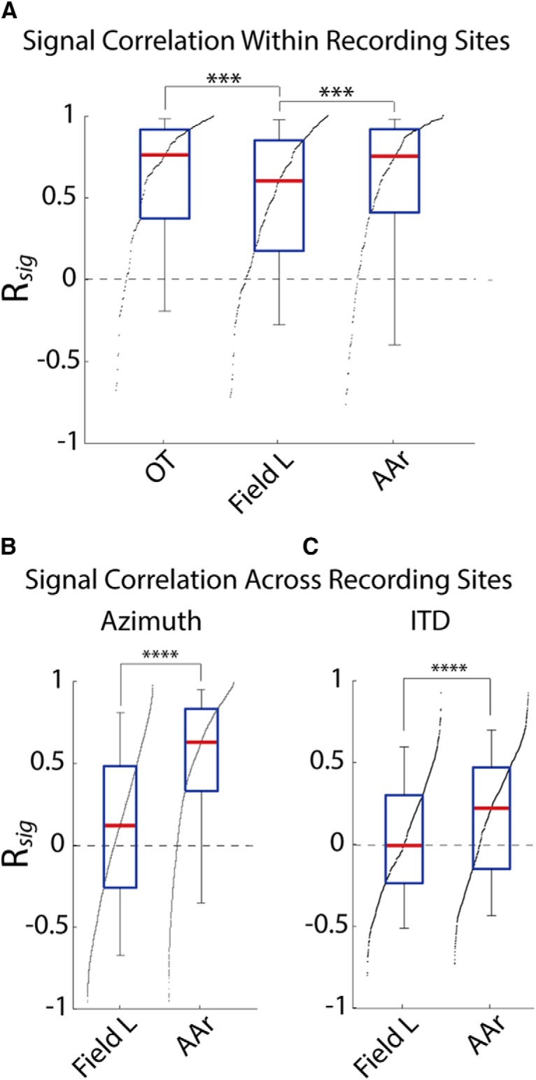
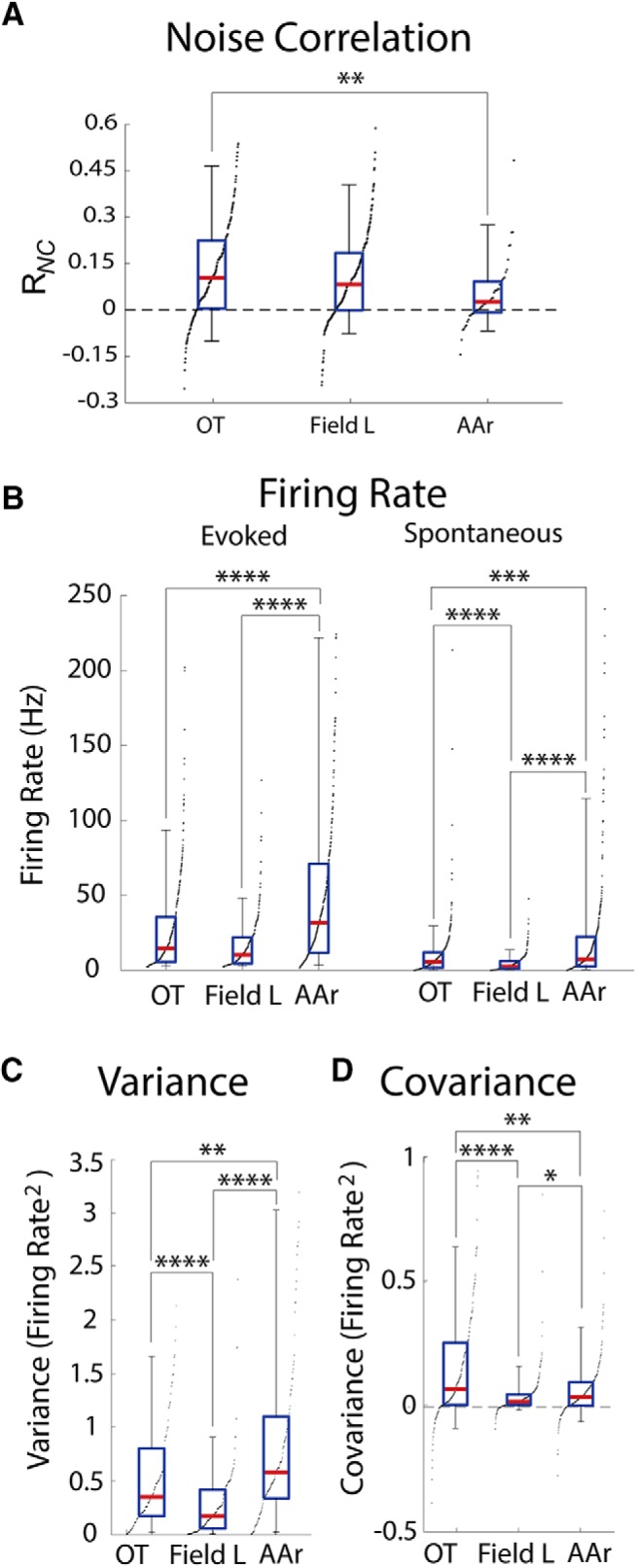
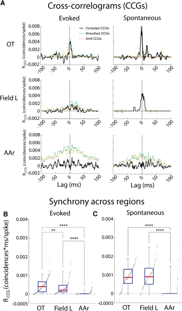
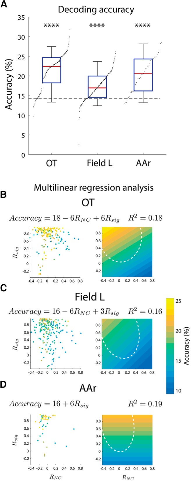
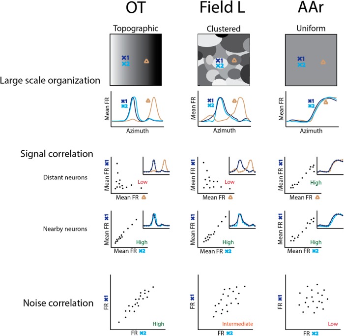
While a topographic map of auditory space exists in the vertebrate midbrain, it is absent in the forebrain. Yet, both brain regions are implicated in sound localization. The heterogeneous spatial tuning of adjacent sites in the forebrain compared to the midbrain reflects different underlying circuitries, which is expected to affect the correlation structure, i.e., signal (similarity of tuning) and noise (trial-by-trial variability) correlations. Recent studies have drawn attention to the impact of response correlations on the information readout from a neural population. We thus analyzed the correlation structure in midbrain and forebrain regions of the barn owl's auditory system. Tetrodes were used to record in the midbrain and two forebrain regions, Field L and the downstream auditory arcopallium (AAr), in anesthetized owls. Nearby neurons in the midbrain showed high signal and noise correlations (R _NC s), consistent with shared inputs. As previously reported, Field L was arranged in random clusters of similarly tuned neurons. Interestingly, AAr neurons displayed homogeneous monotonic azimuth tuning, while response variability of nearby neurons was significantly less correlated than the midbrain. Using a decoding approach, we demonstrate that low R _NC in AAr restricts the potentially detrimental effect it can have on information, assuming a rate code proposed for mammalian sound localization. This study harnesses the power of correlation structure analysis to investigate the coding of auditory space. Our findings demonstrate distinct correlation structures in the auditory midbrain and forebrain, which would be beneficial for a rate-code framework for sound localization in the nontopographic forebrain representation of auditory space.

Figure 1.

Schematic of tectal (blue) and forebrain (red) auditory pathways of the owl’s brain. The auditory midbrain consists of subdivisions of the inferior colliculus: the central core (ICc), lateral shell (ICls), and external nucleus (ICx). The map of auditory space first emerges in ICx. ICx projects to the OT, analog to the superior colliculus. The forebrain pathway originates in projections from the inferior colliculus to the thalamus. The auditory forebrain structure Field L, analog to primary auditory cortex, displays a clustered nontopographic tuning to binaural cues. Field L projects directly to the AAr, analog to the auditory portion of the frontal eye fields. AAr sends projections back onto OT. For clarity, some connections are omitted.

Figure 2.

Azimuth tuning of nearby neurons in OT. A, Spatial receptive field (SpRF) (top) and azimuth tuning curve (bottom) obtained by averaging the SpRF across elevation. B, Peristimulus time histogram (PSTH; top) and raster (bottom) for the spiking activity of the neuron in A responding to sound at the preferred direction (90° azimuth and 0° elevation). C, Example azimuth tuning curves of neurons recorded from the same site. Responses are normalized to facilitate visual comparison. Tuning curves represent mean ± SEM, 20–40 repetitions.

Figure 3.

Azimuth tuning in Field L. A, Example SpRFs (top) and azimuth tuning curves (bottom) of Field L neurons from different recording sites. B, Peristimulus time histogram (PSTH; top) and rasters (bottom) for the spiking activity of the neurons in Afor sounds from the speakers eliciting the maximal response. C, Example azimuth tuning curves of neurons recorded from the same site (different neurons from A, B). Firing rates are normalized to facilitate comparison. Tuning curves represent mean ± SEM, 20–40 repetitions. D, R_sig for azimuth tuning of nearby cells (left) and cells from different recording sites (right). Box plots show median (red line), interquartile range (blue), and 5% and 95% quantiles (whiskers). Black dots indicate the sorted distribution of data points. Asterisks indicate statistical significance (****p < 0.0001; two-tailed Mann–Whitney U test).

Figure 4.

Spatial tuning in AAr. A, Example SpRF (top) and azimuth tuning curve (bottom). B, Peristimulus time histogram (PSTH; top) and rasters (bottom) for the spiking activity of the neuron in A, stimulated by sound from the speaker that elicited the maximal response (20° azimuth and −20° elevation). C, Example azimuth tuning curves of neurons recorded from the same site. Curves show normalized firing (mean ± SEM, 20–40 repetitions). D, Signal correlation for azimuth tuning of nearby cells (left) and cells from different recording sites (right). E, Overlaid azimuth tuning curves of all neurons in the AAr dataset. F, Signal correlation within ipsilateral, frontal, and contralateral azimuth subregions of distant cells. G, Steepness (slope) of azimuth tuning curves within ipsilateral, frontal, and contralateral space. Box plots in D, F, Gshow median (red line), interquartile range (blue), and 5% and 95% quantiles (whiskers). Black dots indicate the sorted distribution of data points. ****p < 0.0001. D, Two-tailed Mann–Whitney U test; F, G, Kruskal-Wallis H test with Dunn’s multiple comparisons correction.

Figure 5.

Comparison of signal correlation across brain regions. A, Signal correlation in nearby cells for azimuth tuning. B, C, Signal correlation across recording sites, for azimuth (B) and ITD (C) tuning. The significantly stronger signal correlation across distant cells in AAr corroborates a more homogeneous tuning than in Field L. Box plots show median (red line), interquartile range (blue), and 5% and 95% quantiles (whiskers). Black dots indicate the sorted distribution of raw values. ***p < 0.001, ****p < 0.0001. A, Kruskal-Wallis H test with Dunn’s multiple comparisons correction; B, C, two-tailed Mann–Whitney U test.

Figure 6.

Comparison of R_NCs. A, R_NCs in OT, Field L, and AAr. B, Average firing rates of OT, Field L, and AAr cells during sound presentation (left) and spontaneous firing (right). C, D, Average variance (C) and covariance (D) in OT, Field L, and AAr neurons. Box plots represent median (red line), interquartile range (blue), and 5% and 95% quantiles (whiskers). Black dots indicate the sorted distribution of raw values. *p < 0.05, **p < 0.01, ***p < 0.001, ****p < 0.0001; Kruskal-Wallis H test with Dunn’s multiple comparisons correction.

Figure 7.

Spike-time synchrony in OT, Field L, and AAr. A, Example CCGs for pairs of evoked (left) and spontaneous (right) responses in OT (top), Field L (middle), and AAr (bottom). The corrected CCGs for individual pairs of neurons (solid black) are overlaid to the smoothed CCG (dashed green) and shifted CCG (dashed orange). The plots for left and right are from the same pair. B, C, Statistical comparison of synchrony across brain regions for evoked (B) and spontaneous (C) spikes. Box plots represent median (red line), interquartile range (blue), and 5% and 95% quantiles (whiskers). Black dots indicate the sorted data; **p < 0.01, ****p < 0.0001; Kruskal-Wallis H test with Dunn’s multiple comparisons correction.

Figure 8.

Decoding of ITD and azimuth from firing rate. A, Decoding accuracy in pairs of simultaneously recorded units in OT, Field L, and AAr. Box plots represent median (red line), interquartile range (blue), and 5% and 95% quantiles (whiskers). Asterisks indicate better than chance level decoding of azimuth (dashed line: 14.92°). Dots are the sorted data points. B–D, left, Decoder performance (colored points) plotted against signal (R_sig) and R_NC for each pair of neurons in OT (B), Field L (C), and AAr (D). Point color indicates level of accuracy (color bar on the right). Right, Linear fit of accuracy data as a function of signal and R_NC. White dashed ellipsoids depict 95% range of signal and R_NCs used for the linear fit, which avoided outliers. Fit functions and R ² values are shown above each plot. Color bar matches all plots (****p < 0.0001; Wilcoxon signed-rank test).

Figure 9.

Summary of findings. Top, Large-scale spatial tuning organization of each region (above) and corresponding schematic tuning curves at recording locations (below) denoted by crosses (X1 and X2 represent nearby sites) and triangles representing a distant site. OT displays a topographic organization of spatial tuning, while Field L is organized in clusters. AAr displays uniform tuning. Middle, Signal correlation for distant (above) and nearby (below) neurons. Tuning curves of distant sites is different in OT (extrapolated from previous descriptions) and Field L but similar in AAr (insets). On the other hand, tuning curves of nearby neurons are similar in all three structures. Scatter plots represent firing rates (FR) of pairs of cells across azimuth plotted against one another, used to calculate signal correlation. Tuning curves are shown in the insets. Bottom, Schematic scatter plots representing the correlated FR variability of nearby cells in OT, intermediate level of FR variability in Field L, and uncorrelated FR variability in AAr.

References

1. Alkire MT, Miller J (2005) General anesthesia and the neural correlates of consciousness. Prog Brain Res 150:229–244. 10.1016/S0079-6123(05)50017-7 - DOI - PubMed
1. Atencio CA, Schreiner CE (2013) Auditory cortical local subnetworks are characterized by sharply synchronous activity. J Neurosci 33:18503–18514. 10.1523/JNEUROSCI.2014-13.2013 - DOI - PMC - PubMed
1. Atencio CA, Shen V, Schreiner CE (2016) Synchrony, connectivity, and functional similarity in auditory midbrain local circuits. Neuroscience 335:30–53. 10.1016/j.neuroscience.2016.08.024 - DOI - PMC - PubMed
1. Averbeck BB, Latham PE, Pouget A (2006) Neural correlations, population coding and computation. Nat Rev Neurosci 7:358–366. 10.1038/nrn1888 - DOI - PubMed
1. Averbeck BB, Lee D (2006) Effects of noise correlations on information encoding and decoding. J Neurophysiol 95:3633–3644. 10.1152/jn.00919.2005 - DOI - PubMed
Publication types
LinkOut - more resources