Logic Modeling in Quantitative Systems Pharmacology

Abstract

Here we present logic modeling as an approach to understand deregulation of signal transduction in disease and to characterize a drug's mode of action. We discuss how to build a logic model from the literature and experimental data and how to analyze the resulting model to obtain insights of relevance for systems pharmacology. Our workflow uses the free tools OmniPath (network reconstruction from the literature), CellNOpt (model fit to experimental data), MaBoSS (model analysis), and Cytoscape (visualization).

Figure 1

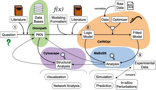
Workflow suggested when applying logic modeling to the study of a biological question. In this tutorial we use Omnipath 48 for signaling database mining, CellNOpt 49 for model fitting, MaBoSS 50 for simulations, and Cytoscape 51 for visualization and network analysis. Different steps of the pipeline include 1) selecting a system and a question of interest and building a first version of the network, 2) choosing a modeling formalism and improving the model with data, and 3) analyzing the model, making predictions and comparing them to experimental data. The dashed arrow indicates a comparison between the results of the analysis and the experimental data. Dotted arrows represent feedback of the results into the modeling pipeline. Rounded boxes represent elements that can be considered part of the different types of the analysis. PKN, prior knowledge network.

Figure 2

(a) Prior knowledge network (PKN) derived from public resources, including interactions connecting nodes which are measured (in blue) or perturbed (stimulated in green and inhibited in red) in the experimental data.57 The network was further expanded to include more components from the apoptotic pathway (p53, Caspase8, and Caspase 9) and Myc for the cell cycle activation and their regulation of Survival. Network layout is generated with Cytoscape.51 (b) Examples of logic rules used to convert the network to a logic model. All other nodes in the model with more than one input edge are modeled with a simple OR gate.

Figure 3

(a) Optimized model with node and edge parameter values represented in grayscale. Dotted lines correspond to compressed nodes and edges which are removed before training the model, as not identifiable from the experimental data. (b) Top panels show four examples of fit of optimal model simulation to experimental values. For each measured phosphoprotein in each experimental condition, color scale is used to represent the mean squared error (MSE). (c) Scatterplot of simulations using the optimal model with respect to experimental data, showing good correlation. (d) Comparison of best model with the results of model optimization after bootstrap (repeated 300 times), network randomization (100 times), and data randomization (300 times) using different scoring metrics, i.e., MSE, coefficient of determination (COD), Pearson correlation (r).

Figure 4

Outputs of MaBoSS simulations with random initial states. (a) Time trajectories of unperturbed model (WT) or model treated with PI3K inhibitor (iPI3K) and mTOR inhibitor (imTOR), with arbitrary time units. (b) Barplot of final state distribution for the unperturbed model. The probability of seven final model states are shown (Caspase 8‐Myc state means that the two variables are present, all the others are 0).

Figure 5

Probability of the node “Survival” predicted by the model for different node inhibitions. Survival probability in the control case (unperturbed model) is marked with a gray line.

Figure 6

Network of synergistic and antagonistic interactions computed for the trained model, with random initial conditions (except for Stress = 0), with Survival as quantitative phenotype. Red triangles represent gain of function alterations and green glyphs represent loss of function alterations. Edges between two alterations show that a combined alteration has a drastic decreasing (in blue) or increasing (in green) effect on the Survival probability when compared to single alterations.

References

-
- Swinney, D.C. & Anthony, J. How were new medicines discovered? Nat. Rev. Drug Discov. 10, 507–519 (2011). - PubMed
- Iorns, E. , Lord, C.J. , Turner, N. & Ashworth, A. Utilizing RNA interference to enhance cancer drug discovery. Nat. Rev. Drug Discov. 6, 556–568 (2007). - PubMed
- Shembekar, N. , Chaipan, C. , Utharala, R. & Merten, C.A. Droplet‐based microfluidics in drug discovery, transcriptomics and high‐throughput molecular genetics. Lab Chip 16, 1314–1331 (2016). - PubMed
Publication types
MeSH terms
Substances
LinkOut - more resources
Full Text Sources
Other Literature Sources