A novel ultra high-throughput 16S rRNA gene amplicon sequencing library preparation method for the Illumina HiSeq platform

Abstract

Background: Advances in sequencing technologies and bioinformatics have made the analysis of microbial communities almost routine. Nonetheless, the need remains to improve on the techniques used for gathering such data, including increasing throughput while lowering cost and benchmarking the techniques so that potential sources of bias can be better characterized.

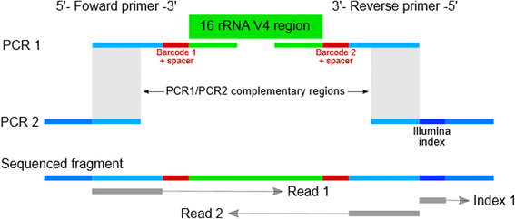
Methods: We present a triple-index amplicon sequencing strategy to sequence large numbers of samples at significantly lower c ost and in a shorter timeframe compared to existing methods. The design employs a two-stage PCR protocol, incorpo rating three barcodes to each sample, with the possibility to add a fourth-index. It also includes heterogeneity spacers to overcome low complexity issues faced when sequencing amplicons on Illumina platforms.

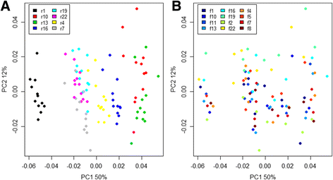
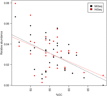
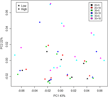
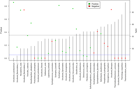
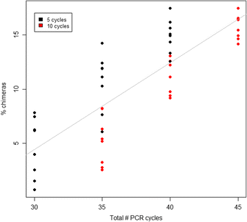
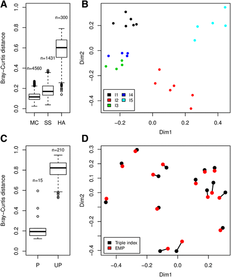
Results: The library preparation method was extensively benchmarked through analysis of a mock community in order to assess biases introduced by sample indexing, number of PCR cycles, and template concentration. We further evaluated the method through re-sequencing of a standardized environmental sample. Finally, we evaluated our protocol on a set of fecal samples from a small cohort of healthy adults, demonstrating good performance in a realistic experimental setting. Between-sample variation was mainly related to batch effects, such as DNA extraction, while sample indexing was also a significant source of bias. PCR cycle number strongly influenced chimera formation and affected relative abundance estimates of species with high GC content. Libraries were sequenced using the Illumina HiSeq and MiSeq platforms to demonstrate that this protocol is highly scalable to sequence thousands of samples at a very low cost.

Conclusions: Here, we provide the most comprehensive study of performance and bias inherent to a 16S rRNA gene amplicon sequencing method to date. Triple-indexing greatly reduces the number of long custom DNA oligos required for library preparation, while the inclusion of variable length heterogeneity spacers minimizes the need for PhiX spike-in. This design results in a significant cost reduction of highly multiplexed amplicon sequencing. The biases we characterize highlight the need for highly standardized protocols. Reassuringly, we find that the biological signal is a far stronger structuring factor than the various sources of bias.

Keywords: 16S rRNA gene amplicon sequencing; Benchmarking; Chimera formation; Environmental sequencing; Illumina library preparation; Indexed PCR; Mock community; PCR bias.

Fig. 1

Triple indexing design. The triple indexing strategy incorporates two PCR steps. During the first PCR (PCR1), the template sequence of interest is targeted and amplified (green). The primers for this reaction also contain an indexing sequence and a heterogeneity spacer sequence (red), and a partial Illumina adapter (blue). A second PCR (PCR2) allows for the introduction of a third indexing sequence (dark blue) as well as completion of the Illumina sequencing adapter

Fig. 2

Relative abundances of the 33 bacterial species in the mock community sample estimated from both the MiSeq (dataset 1, n = 96) and HiSeq (dataset 4, n = 24) data (Additional file 4: Table S3, Additional file 7: Table S6). Species abundance estimates are shown side-by-side with MiSeq estimates labeled ‘MS’ and HiSeq estimates labeled ‘HS’. For enhanced visualization, each pair of colored bars (blue or white) depicts the estimated relative abundances for one species. The dotted red line shows the relative abundance expectation given perfectly equal blending. Each box represents the interquartile range while the whiskers represent 1.5 times the interquartile range. Points outside the whiskers represent outliers

Fig. 3

Scores plot based on a principal component analysis model computed from the matrix of species relative abundances from dataset 1 (Additional file 4: Table S3). a. Samples are colored according to the reverse primer used for PCR1. b. Samples are colored according to the forward primer used for PCR1. In both a and b, the first two dimensions, explaining 62% of the total variance, are shown

Fig. 4

Relationship between mean relative abundance estimates and GC percentage for datasets 1 and 4. There is a significant negative linear relationship for both the MiSeq (p = 0.002, n = 96, Additional file 4: Table S3) and HiSeq (p = 0.012, n = 24, Additional file 7: Table S6) data. Estimates drop by 0.18 and 0.16% for each 1% increase in GC content for the MiSeq and HiSeq estimates, respectively

Fig. 5

Scores plot based on a principal component analysis model computed from the matrix of species relative abundances from dataset 3 (Additional file 6: Table S5). Samples are colored according to PCR1 and PCR2 cycle regime, with the number of cycles indicated in the legend (PCR1 + PCR2). Filled dots and triangles represent samples prepared with tenfold difference in input DNA template concentration used for PCR1. The first two dimensions, explaining 65% of the total variance, are shown

Fig. 6

Statistical significance and direction of relationships between estimated relative abundances of sequence reads and PCR cycle number (Additional file 18: Figure S9) in dataset 3. The dots represent p values from linear regression models, with green and red representing positive and negative relationships, respectively. The species are ordered according to the GC content on the sequenced fragment (vertical lines). The dotted blue lines signifies the significance threshold of p = 0.05 (left axis), while the dotted black line represents the mean GC percentage (right axis)

Fig. 7

Relationship between PCR cycle number and chimeric sequence formation in dataset 3. The combined numbers of PCR1 and PCR2 amplification cycles are indicated on the x-axis. Black and red dots indicate samples amplified using 5 and 10 cycles for PCR2, respectively. A highly significant linear relationship (p < <0.001, linear regression model) was observed. The effects were primarily related to the PCR1 cycle number, e.g., samples undergoing 35 cycles (25 cycle PCR1 and 10 cycles PCR 2) had less chimeras than samples undergoing 35 cycles (30 cycles PCR1 and 5 cycles PCR2)

Fig. 8

a. Pairwise Bray-Curtis distances for the mock community (MC, dataset 1, Additional file 4: Table S3), standardized sample (SS, dataset 5, Additional file 8: Table S7), and healthy adult (HA, dataset 6, Additional file 9: Table S8) group. Each box represents the interquartile range while the whiskers represent 1.5 times the interquartile range. Points outside the whiskers represent outliers. The number of pairwise distances for each group is indicated over the boxes. b. Multidimensional scaling (MDS) plot showing clustering of 25 samples taken from 5 healthy adult volunteers (dataset 6, Additional file 9: Table S8). Sample origin is indicated by color (individual 1–5). The stress value of the MDS model was 13.2%, indicating a good fit. c. Pairwise Bray-Curtis distances for the 15 samples sequenced using 2 different library preparation methods (dataset 7, Additional file 10, Table S9). The leftmost box shows distances between identical samples (P = paired), while the box on the right shows the distances for non-identical samples (UP = unpaired). d Multidimensional scaling plot showing clustering of the 15 samples sequenced using 2 different library preparation methods (dataset 7, Additional file 10, Table S9). Paired samples, i.e., identical samples sequences using different techniques, are joined by black lines

References

-
- Low-diversity sequencing on the Illumina HiSeq platform (Illumina Technical Note 770-2014-035). Illumina. 2014. http://www.illumina.com/documents/products/technotes/technote-hiseq-low-... Accessed June 2016.
- Kozich JJ, Westcott SL, Baxter NT, Highlander SK, Schloss PD. Development of a dual-index sequencing strategy and curation pipeline for analyzing amplicon sequence data on the MiSeq Illumina sequencing platform. Appl Environ Microbiol. 2013;79:5112–20. doi: 10.1128/AEM.01043-13. - DOI - PMC - PubMed
Publication types
MeSH terms
Substances
LinkOut - more resources
Full Text Sources
Other Literature Sources
Miscellaneous