Dynamic graph metrics: Tutorial, toolbox, and tale

Abstract

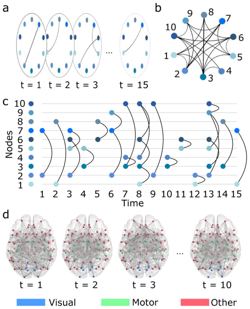
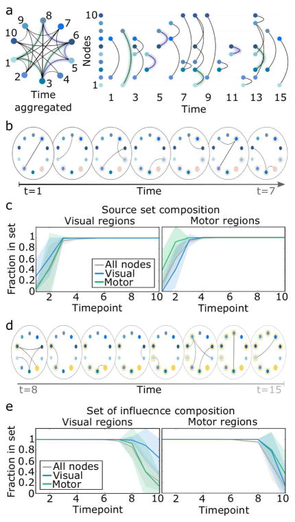
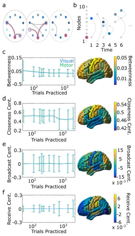
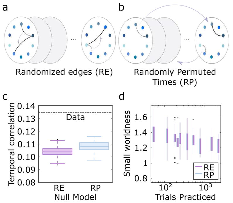
The central nervous system is composed of many individual units - from cells to areas - that are connected with one another in a complex pattern of functional interactions that supports perception, action, and cognition. One natural and parsimonious representation of such a system is a graph in which nodes (units) are connected by edges (interactions). While applicable across spatiotemporal scales, species, and cohorts, the traditional graph approach is unable to address the complexity of time-varying connectivity patterns that may be critically important for an understanding of emotional and cognitive state, task-switching, adaptation and development, or aging and disease progression. Here we survey a set of tools from applied mathematics that offer measures to characterize dynamic graphs. Along with this survey, we offer suggestions for visualization and a publicly-available MATLAB toolbox to facilitate the application of these metrics to existing or yet-to-be acquired neuroimaging data. We illustrate the toolbox by applying it to a previously published data set of time-varying functional graphs, but note that the tools can also be applied to time-varying structural graphs or to other sorts of relational data entirely. Our aim is to provide the neuroimaging community with a useful set of tools, and an intuition regarding how to use them, for addressing emerging questions that hinge on accurate and creative analyses of dynamic graphs.

FIG. 1

Visualizations of dynamic networks. (a) Stacked static network representation of a dynamic network on ten nodes. (b) Time-aggregated graph of the dynamic network in (a). Any two nodes that are connected at any time in (a) are connected in this graph. (c) Visualization of the network in (a) as contacts across time. (d) Dynamic network of one individual during a motor learning task [50]. Green regions correspond to a functional module composed of motor areas, blue regions correspond to a functional module composed of visual regions, and red regions correspond to areas that were not in either the motor module or the visual module. Toolbox functions used to create this figure: randomDN, plotArcNetwork, plotDNarc.

FIG. 2

Time respecting paths. (a) (Left) Time aggregated network from Fig. 1b with green and blue paths highlighted. (Right) Contact sequence plot from Fig. 1c with green and blue paths highlighted. (b) The source set of the peach node indicated with a peach ring. (c) Composition of the source set of nodes from the visual (left) and motor (right) modules of our example empirical fMRI data set, depicted across time. The gray line indicates the fraction of all nodes in the source set, while the blue and green lines represent the fraction of the visual and motor nodes within the source set, respectively. (d) Illustration of the set of influence (t − 8) of the gold node. Nodes within this set indicated with a gold ring at the time at which they can first be reached by the gold node. (e) Composition of the set of influence calculated from nodes within the visual (left) and motor (right) groups. As in (c), the fraction of all regions (gray), visual regions (blue), and motor regions (green) are plotted against time. Solid lines in (c) and (e) mark the average over subjects and trials, and shaded regions represent two standard deviations from this average. Toolbox functions used to create this figure: sourceSet, setOfInfluence.

FIG. 3

Centrality in dynamic networks. (a) Time window of the model network shown in Fig. 1a–c highlighting the fastest paths that pass through the maroon node, and therefore affect its betweenness centrality. (b) Schematic of closeness centrality for the maroon node in the model network. Closeness centrality measures the speed at which a node can reach all others: the time at which other nodes are first reached by node 2 determines its closeness centrality. Nodes are shown in color at the earliest time they are reached by node 2. (c–f ) An illustration of the notions of centrality for our example empirical fMRI data shown in Fig. 1d. (c) (Left) Betweenness centrality for visual (blue) and motor (green) regions as a function of the number of trials practiced. (Right) Averaged betweenness centrality scores across trials practiced for each brain region. (d) Closeness centrality for visual and motor regions during learning (left), and (right) averaged over the number of trials as in (c). (e) Broadcast centrality for visual and motor regions during learning (left), and the same values now averaged over all trials (right). (f ) Receive centrality for visual and motor regions during learning (left), and the same values now averaged over all trials (right). Error bars indicate two standard deviations from the mean over subjects and trials practiced. Toolbox functions used to create this figure: betweenessCentrality, closenessCentrality, broad castReceiveCentrality.

FIG. 4

Null models and their utility in measuring small-worldness in dynamic graphs. (a) Schematic of the edge rewiring process for the randomized edges (RE) model. (b) Schematic of the randomly permuted times (RP) model where contact times are permuted uniformly at random. (c) Temporal correlation coefficients for one session of a participant in the study (black dashed line), and the 100 runs of the RE and RP model created from this dynamic network. (d) Small-worldness calculations using either the RE (purple) or RP (blue) null model. Toolbox functions used include randomized-Edges, randPermutedTimes, temporalCorrelation, and temporalSmallWorldness.

FIG. 5

Metrics associated with dynamic community structure. (a) Example dynamic network with a community partition: an assignment of nodes to communities (densely intraconnected groups of nodes) as a function of time. Node community assignments are shown both within a sequence of graphs (top), and as a heatmap (bottom). Examples of nodes with high (orange) and low (blue) values for associated metrics: (b) flexibility, (c) promiscuity, and (d) cohesion.

References

-
- Breakspear M. Dynamic models of large-scale brain activity. Nat Neurosci. 2017;20:340–352. - PubMed
- Villoslada P, Steinman L, Baranzini SE. Systems biology and its application to the understanding of neurological diseases. Ann Neurol. 2009;65:124–139. - PubMed
- Cooper RP, Shallice T. Cognitive neuroscience: the troubled marriage of cognitive science and neuroscience. Top Cogn Sci. 2010;2:398–406. - PubMed
Publication types
MeSH terms
Grants and funding
LinkOut - more resources
Full Text Sources
Other Literature Sources