Imaging at ultrahigh magnetic fields: History, challenges, and solutions

Abstract

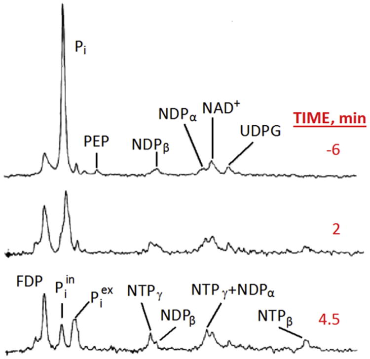
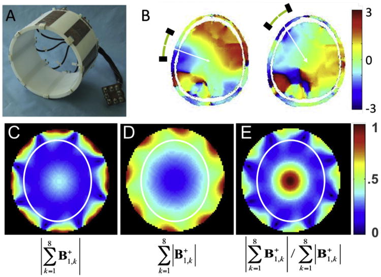
Following early efforts in applying nuclear magnetic resonance (NMR) spectroscopy to study biological processes in intact systems, and particularly since the introduction of 4 T human scanners circa 1990, rapid progress was made in imaging and spectroscopy studies of humans at 4 T and animal models at 9.4 T, leading to the introduction of 7 T and higher magnetic fields for human investigation at about the turn of the century. Work conducted on these platforms has provided numerous technological solutions to challenges posed at these ultrahigh fields, and demonstrated the existence of significant advantages in signal-to-noise ratio and biological information content. Primary difference from lower fields is the deviation from the near field regime at the radiofrequencies (RF) corresponding to hydrogen resonance conditions. At such ultrahigh fields, the RF is characterized by attenuated traveling waves in the human body, which leads to image non-uniformities for a given sample-coil configuration because of destructive and constructive interferences. These non-uniformities were initially considered detrimental to progress of imaging at high field strengths. However, they are advantageous for parallel imaging in signal reception and transmission, two critical technologies that account, to a large extend, for the success of ultrahigh fields. With these technologies and improvements in instrumentation and imaging methods, today ultrahigh fields have provided unprecedented gains in imaging of brain function and anatomy, and started to make inroads into investigation of the human torso and extremities. As extensive as they are, these gains still constitute a prelude to what is to come given the increasingly larger effort committed to ultrahigh field research and development of ever better instrumentation and techniques.

Fig. 1

145.7 MHz (8.46 T) ³¹P spectra of anaerobic E. coli cells in suspension, initially without a carbon source. At time 0, glucose was added to the suspension. Each spectrum represents 200 averages collected in 2 min. NDP and NTP, Nucleotide di- and tri-phosphate respectively; PEP, phosphoenolpyruvate; FDP, fructose di-phosphate; P_i inorganic phosphate representing both intracellular and extracellular contributions; ${\mathrm{P}}_{\mathrm{i}}^{\text{ex}}$, ${\mathrm{P}}_{\mathrm{i}}^{\text{in}}$ extra and intracellular inorganic phosphate. Adapted from Ugurbil et al. (1978b).

Fig. 2

(A) and (B): Early 4 T brain images published from Siemens (Barfuss et al., 1988, 1990); (C) 4 T MDEFT image of human brain obtained at the CMRR (Ugurbil et al., 1993; Lee et al., 1995); (D) Contemporary 7 T brain image in coronal section showing hippocampal formation (Henry et al., 2011); and (E) 7 T image in the human torso displaying a coronal cut through the human heart (Erturk et al., 2017a).

Fig. 3

Early functional images produced in the human brain, obtained at (A) 1.5 T (Kwong et al., 1992), and (B) 4 T from CMRR (Ogawa et al., 1992). (C) The anatomical image of slice that was used for the functional imaging in (B), with the cortical surface outlined in red. (D) The same image as (B) but with the same red line outlining the cortical surface superimposed on it.

Fig. 4

A Fax (top) and an email (lower) from David Rayner dated 03 August 1995 and 01 April 96, respectively, discussing the 7 T initiative. The approximate pricing supplied is blanked out. The color markings in the 1996 email identify our deliberations in CMRR at the time. Ultimately we decided on the 7.0/900-cm bore magnet; this design was employed on all 7 T systems installed until 2011 when two new, actively shielded 7 T magnets with 830 and 900 cm bore diameters were developed.

Fig. 5

SNR measurements from fully relaxed gradient echo images acquired using the same acquisition parameters and homogeneous TEM volume coils of identical dimensions at 4 T (A), and at 7 T (B). Averaged, regional SNR values are shown on the images. Average 7 T/4 T SNR ratios are listed beneath the SNR data on the 7 T image. (C) shows a figure from Maxwell model with calculated 7 T/4 T SNR ratios, which are consistent with experimental data.

Fig. 6

Transmit B1 magnitude in the human head at 7 T, generated by a volume TEM coil. The color code is proportional to μTesla/V.

Fig. 7

2D plots of instantaneous transverse jB1j for 7 T at progressing points in phantoms with different conductivities: (a) ωt = 0 S/m, (b) ωt = 0.26 S/m, and (c) ωt = 0.67 S/m. The intensity profiles along the horizontal centerlines are also shown on the right of the 2D plots. The surface coil position is indicated by two small dots on the left side of the phantom. Since the temporal B1 strength varies greatly among these three cases, the signal intensities of temporal points are normalized individually for each conductivity condition in order to visualize the temporal change for all the conditions clearly.

Fig. 8

Electromagnetic simulations of the transmit B₁ field in a body RF coil at 7 T. The coil produces a homogenous B₁ when empty (top figure) but not when loaded with the human body (lower figure) (work by Jinfeng Tian and Thomas Vaughan, CMRR).

Fig. 9

Eight channel transmit/receive RF coil (A) and experimental relative phases measured in the human head from two different individual elements of this coil (B). Lower row shows experimentally measured transmit B₁ magnitude in a cylindrical “phantom” when the individual transmit B₁ vectors from each channel are first experimentally determined, transmitting one channel at a time and receiving with all channels, and subsequently are added according to the constructs shown below each figure (the color code is in arbitrary units) The white ellipse in C, D, and E depicts approximate boundaries of a human head. Adapted from (Van de Moortele et al., 2005).

Fig. 10

Sixteen channel pTx pulse design for a multiband RF pulse that excites two slices simultaneously in the human brain at 7 T. The L shaped curve quantifies tradeoffs, in this specific case, between total RF energy of the RF pulse and excitation errors (i.e., root mean square error (RMSE)). The crossing between the horizontal and vertical dashed lines, labeled “Same fidelity” and “Same energy”, identify the performance of the same coil operated in a circularly polarized mode. Adapted from Wu et al. (2013).

Fig. 11

Performance of one-spoke (dashed) and two-spoke (solid) pTx pulses to image the kidneys, and the heart. L-curves display tradeoff between excitation error (NRMSE) and resulting peak local SAR for 7.0 T and 10.5 T arrays when designing the pTx pulses with explicit local SAR constraint. Adapted from Erturk et al. (2017b).

Fig. 12

7 T gradient recalled echo (FLASH) image of a single slice in the human head with the same in-plane resolution but with two different slice thickness and hence, different voxel volumes. Arrows in the 5 mm slice point to regions of signal reduction or complete loss due to B₀ inhomogeneities near air filled cavities in the human head. These losses are recovered in the higher resolution, 1 mm thick slice, image.

Fig. 13

Parallel imaging (SENSE) performance for different object size and field magnitude. Simulation shows the log of g-factor as a function of reduction factor R and magnetic field magnitude. Adapted from Wiesinger et al. (2004, .

Fig. 14

7 T Gradient Recalled Echo EPI images obtained with a head gradient, a 32 channel receive coil, and 4-fold acceleration along the phase encode direction. Nominal resolution = 0.75 mm isotropic; 128 slices; echo spacing = 0.67 ms; 256 × 256 matrix; partial Fourier pf = 6/8; TE = 20 ms; TR = 6 s. Right column displays a blowup of 4 of the slices.

Fig. 15

Extravascular relaxation rate changes for R₂ (solid line) and R₂* (dashed line) (equal to 1/T₂, and 1/T₂*, respectively) induced by simulated blood vessels with a magnetic susceptibility difference between blood vessel interior and exterior (basis of extravascular BOLD effect), shown as a function of blood vessel radius (horizontal axis, log scale) and magnetic susceptibility induced different frequency shifts (in Hz) across the blood vessel. The numbers 32, 48, and 64 Hz correspond to increasing magnetic field strength B₀ at a constant deoxyhemoglobin concentration (∼3, 5, and 7 T at physiological conditions) or increasing deoxyhemoglobin concentration at a constant B₀. GE = Gradient Echo, SE = spin echo. Adapted from Uludag and Ugurbil (2015).

Fig. 16

Functional Contrast-to-Noise Ratio (fCNR) for SE BOLD fMRI, normalized to the value at 1.5 T. Calculated using Eq. (1) with the parameter β set to 1. These plots are valid only in the limit where the noise in the fMRI time series is dominated by thermal noise of the images, which is the case for example, for high resolution imaging at the level of cortical columns and layers. Plots generated by Uludağ, K. using data from Uludag et al. (2009).

Fig. 17

Functional maps of orientation and ocular dominance columns in the human brain. Obtained at 7 T using SE fMRI. Adopted from Yacoub et al. (2008).

Fig. 18

Ocular dominance column functional images obtained either by Spin Echo (SE) or Gradient Echo (GRE) fMRI on two separate occasions on the same individual. Each voxel is labeled with either blue or red color if it is reproducibly assigned to same eye on the two different occasions. Thus the maps shown depict the patterns induced by stimulation of one eye versus the other, as well as their reproducibility in a single subject on the two different occasions. Adapted from Yacoub et al. (2007).

Fig. 19

Functional mapping frequency selectivity in the auditory pathway at 7 T. Adapted from Formisano et al. (2003), De Martino et al., 2013a,, Moerell et al., 2015, and De Martino et al., 2015.

Fig. 20

Angle between surface tangent and fiber orientations at the inflated WM/GM boundary surface for the same subject scanned at 3 and 7 T with the respective HCP protocols. For every surface vertex, the maximum dot product between fiber orientations (with volume fraction f > 5%) at this location and the surface normal is computed. This is then converted to the color-code angle shown on the inflated surface. Blue perpendicular, red parallel. From Sotiropoulos et al. (2013).

References

1. Abduljalil A, Kangarlu A, Robitaille PML. Experimental Nuclear Magnetic Resonance Conference (ENC) Orlando, FL: 1999. Ultra-High field magnetic resonance imaging; p. 110.
1. Ackerman JJ, Bore PJ, Gadian DG, Grove TH, Radda GK. N.m.r studies of metabolism in perfused organs. Philos Trans R Soc Lond B Biol Sci. 1980a;289:425–436. - PubMed
1. Ackerman JJ, Grove TH, Wong GG, Gadian DG, Radda GK. Mapping of metabolites in whole animals by 31P NMR using surface coils. Nature. 1980b;283:167–170. - PubMed
1. Adriany G, Auerbach EJ, Snyder CJ, Gozubuyuk A, Moeller S, Ritter J, Van de Moortele PF, Vaughan T, Ugurbil K. A 32-channel lattice transmission line array for parallel transmit and receive MRI at 7 tesla. Magn Reson Med. 2010a;63:1478–1485. - PMC - PubMed
1. Adriany G, Gözübüyük A, Ritter J, Snyder C, Van de Moortele PF, Moeller S, Vaughan JT, Ugurbil K. A 32 channel lattice transmission line array for parallel MRI. Proc Int Soc Mag Reson Med. 2006;14:126. - PMC - PubMed
Publication types