Modeling polymorphic transformation of rotating bacterial flagella in a viscous fluid

Abstract

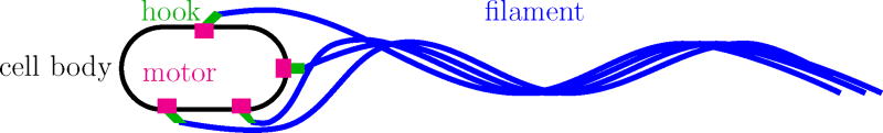
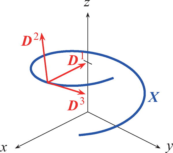
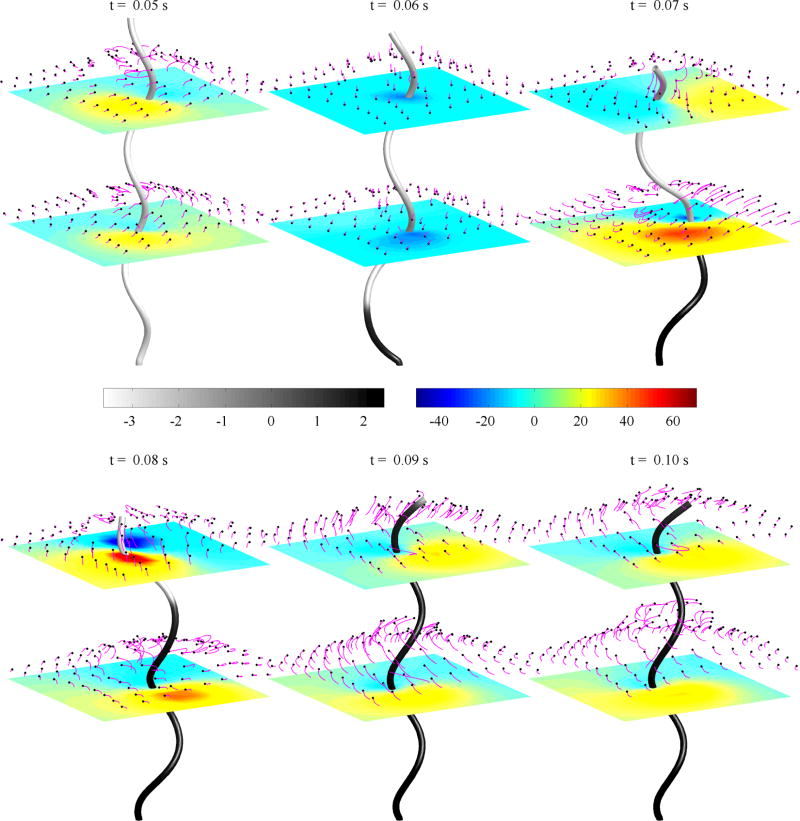
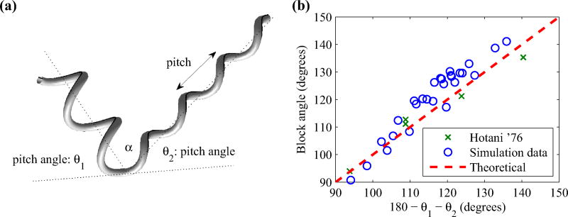
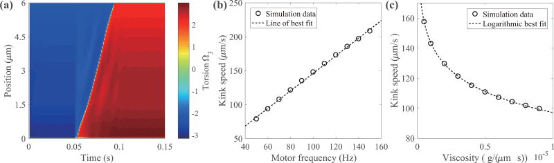
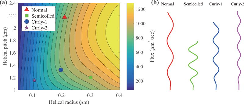
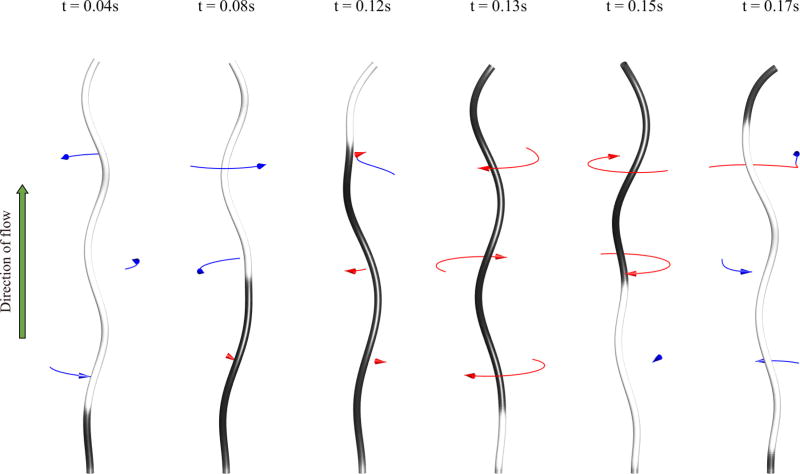
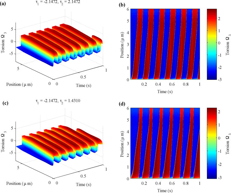
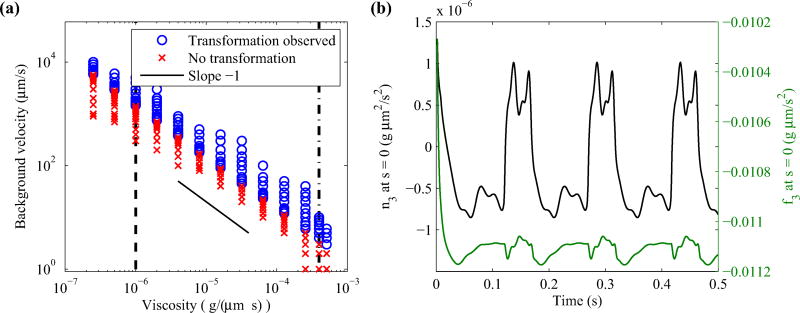
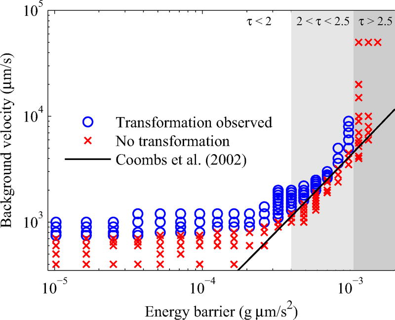
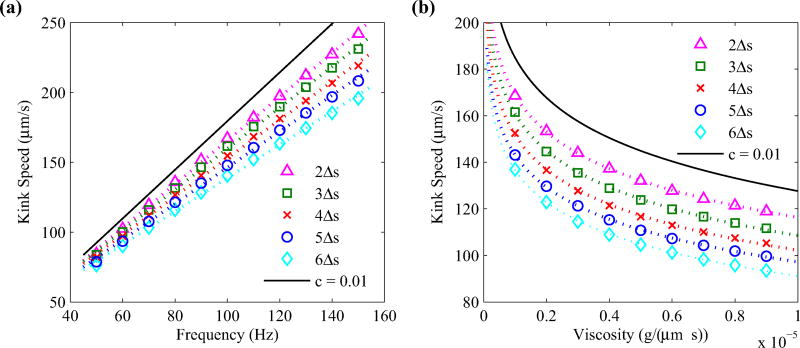
The helical flagella that are attached to the cell body of bacteria such as Escherichia coli and Salmonella typhimurium allow the cell to swim in a fluid environment. These flagella are capable of polymorphic transformation in that they take on various helical shapes that differ in helical pitch, radius, and chirality. We present a mathematical model of a single flagellum described by Kirchhoff rod theory that is immersed in a fluid governed by Stokes equations. We perform numerical simulations to demonstrate two mechanisms by which polymorphic transformation can occur, as observed in experiments. First, we consider a flagellar filament attached to a rotary motor in which transformations are triggered by a reversal of the direction of motor rotation [L. Turner et al., J. Bacteriol. 182, 2793 (2000)10.1128/JB.182.10.2793-2801.2000]. We then consider a filament that is fixed on one end and immersed in an external fluid flow [H. Hotani, J. Mol. Biol. 156, 791 (1982)10.1016/0022-2836(82)90142-5]. The detailed dynamics of the helical flagellum interacting with a viscous fluid is discussed and comparisons with experimental and theoretical results are provided.

FIG. 1

A schematic showing the physiology of an E. coli cell. The flagellar filaments are randomly distributed along the cell body. Each filament is attached to a rotary motor via a flexible hook.

FIG. 2

An illustration of the parametrization of the flagellar filament. The centerline of the flagellum is parameterized by X(s,t) and its orientation is determined by an orthonormal triad {D¹(s,t), D²(s,t), D³(s,t)}.

FIG. 3

The regularized δ function for various smoothing parameter values of c.

FIG. 4

Snapshots of a bistable helix with τ₁ = −2.1472 µm⁻¹ and τ₂ = 1.4310 µm⁻¹, rotating at 100 Hz. The shade of the rod indicates the torsion value where gray is negative (left-handed) and black is positive (right-handed). The horizontal planes show the vertical velocity of the fluid and the markers shown in magenta are passive fluid tracers.

FIG. 5

A schematic diagram of the block angle α formed by a kink in the helical filament (left) and estimated block angles from our simulations for various helical shapes (right). Simulation results and experimental data from Hotani [52] are in good agreement.

FIG. 6

Torsion along the filament over time (left) and kink propagation speed plotted against motor rotation frequency (middle) and fluid viscosity (right). The intrinsic twist values are given as τ₁ = −2.1472 µm⁻¹ and τ₂ = 2.1472 µm⁻¹. The left panel illustrates how torsion changes over time at the rotating frequency of 100 Hz. The negative value (blue) of torsion corresponds to the left-handed helix and the positive value (red) corresponds to the right-handed helix. The kink speed is estimated as the slope of the curve where the filament is torsion-free. The middle and right panels show that the kink speed is approximately proportional to the motor frequency and decreases logarithmically with increasing fluid viscosity, respectively.

FIG. 7

Mean fluid flux driven by a helical flagellum rotating at 100 Hz for various pitches and radii. The markers on the left panel denote the mean flux for four helical shapes commonly observed in nature [11,17], which are shown on the right.

FIG. 8

Simulation of an experiment by Hotani [17] using intrinsic torsion values τ₁ = −2.1472 µm⁻¹ and τ₂ = 1.4310 µm⁻¹. Fluid (water) is flowing upward at 2000 µm/s. The shade of the rod indicates the torsion value where gray is negative (left-handed) and black is positive (right-handed). The arrows indicate CW (red) or CCW (blue) rotation and their length is proportional to the motion over the previous 0.008 s.

FIG. 9

Values of torsion Ω₃ from simulations of Hotani’s experiment plotted against time t and filament position s. The negative value (blue) of torsion corresponds to the left-handed helix and the positive value (red) corresponds to the right-handed helix. The intrinsic torsion values used are τ₁ = −2.1472 µm⁻¹, τ₂ = 2.1472 µm⁻¹ (top) and τ₁ = −2.1472 µm⁻¹, τ₂ = 1.4310 µm⁻¹ (bottom). The fluid viscosity is 0.01 × 10⁻⁴ g/(µm · s). The background flow speed is set to 2000 µm/s.

FIG. 10

(Left) Observed handedness change for various background flow velocity and fluid viscosity. The vertical dashed line and the dashed-dot line denote the viscosity of water and methylcellulose, respectively. Both axes are plotted on a log scale. (Right) Time evolution of n₃ and f₃ at the motor for flow speed 2000 µm/s. In both plots, the intrinsic torsion is set to τ₁ = −2.1472 µm⁻¹ and τ₂ = 1.4310 µm⁻¹.

FIG. 11

Background flow velocity plotted against the energy barrier $H=\frac{a_3}{4}{\tau }^4$ for the symmetric twist energy τ = −τ₁ = τ₂. The result by Coombs et al. (solid curve) was scaled to fit the data. Both axes are plotted on a log scale.

FIG. 12

Kink propagation speed plotted against motor rotation frequency (left) and fluid viscosity (right) for various regularization parameters c = 2Δs, …, 6Δs. Here, Δs = 0.03 µm, and intrinsic twist values are set to τ₁ = −2.1472 µm⁻¹ and τ₂ = 2.1472 µm⁻¹. The dotted lines on the left panel denote the lines of best fit, and the dotted curves on the right panel denote a logarithmic best fit curves. The solid curve in each panel estimates the result for c = 0.01 µm based on the best fit parameters.

References

-
- Lauga E. Annu. Rev. Fluid Mech. 2016;48:105.
- Li C, Motaleb A, Sal M, Goldstein SF, Charon NW. J. Mol. Microbiol. Biotechnol. 2000;2:345. - PubMed
- McBride MJ. Annu. Rev. Microbiol. 2001;55:49. - PubMed
- Weibull C. In: The Bacteria: A Treatise on Structure and Function. Gunsalus IC, Stanier RY, editors. Vol. 1. Academic Press; New York: 1960. pp. 153–205.
- Berg HC. Annu. Rev. Biochem. 2003;72:19. - PubMed
MeSH terms
Substances
Grants and funding
LinkOut - more resources
Full Text Sources
Other Literature Sources