Dynamics of genomic innovation in the unicellular ancestry of animals

Abstract

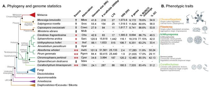
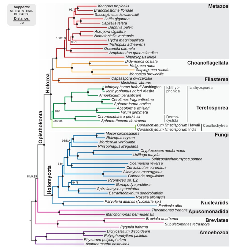
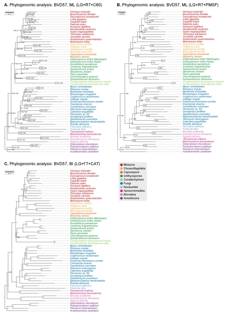
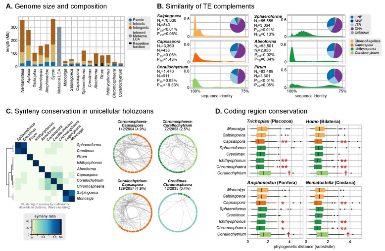
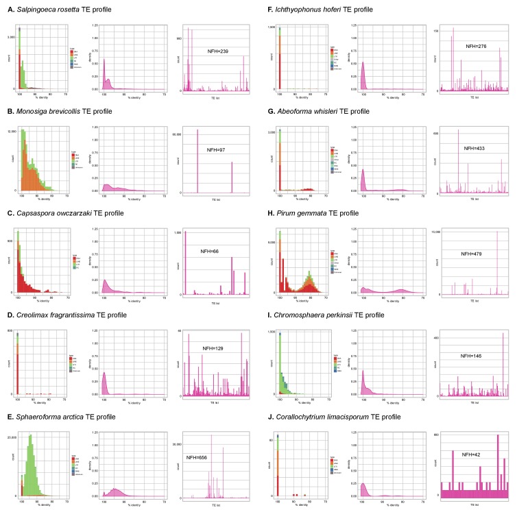
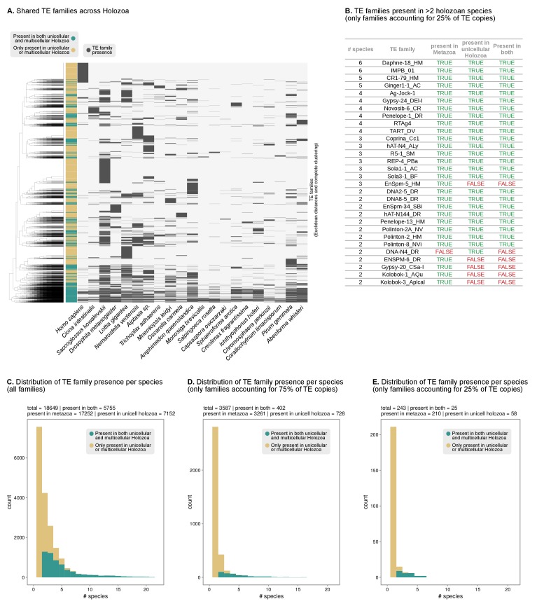
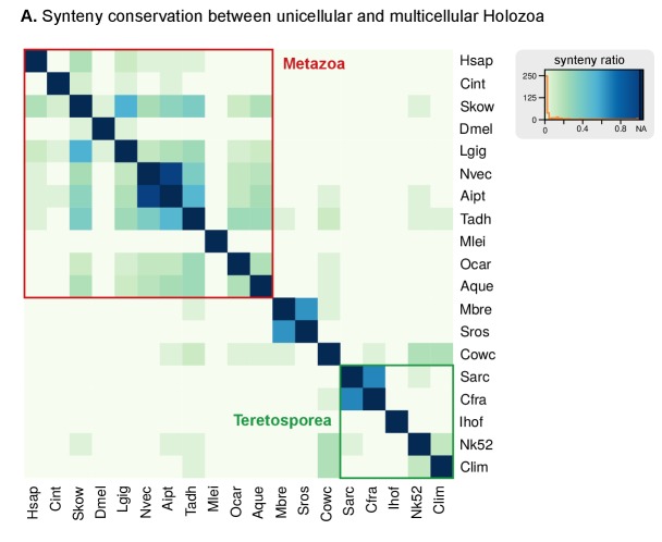
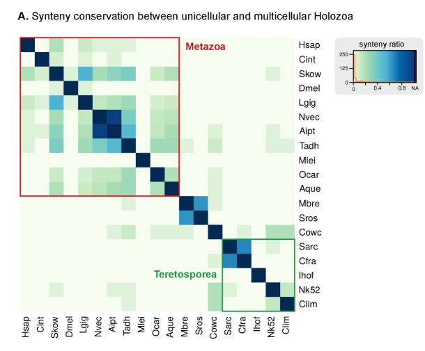
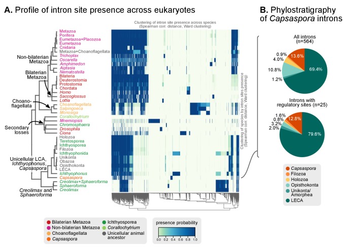
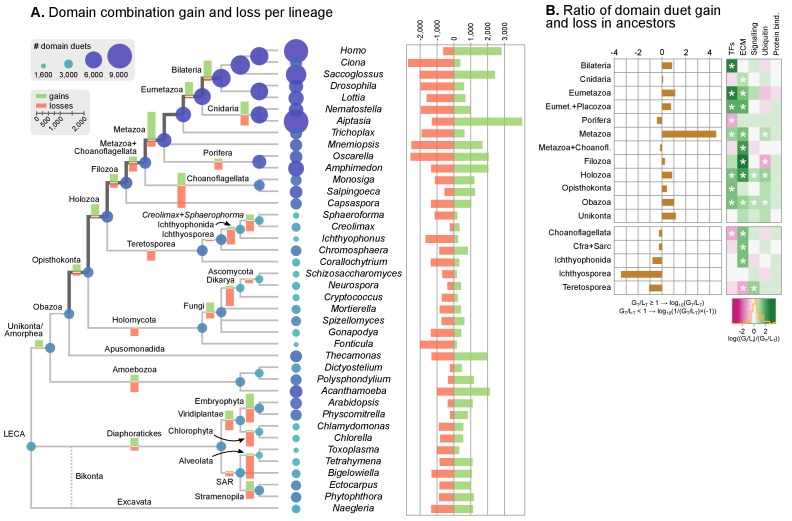
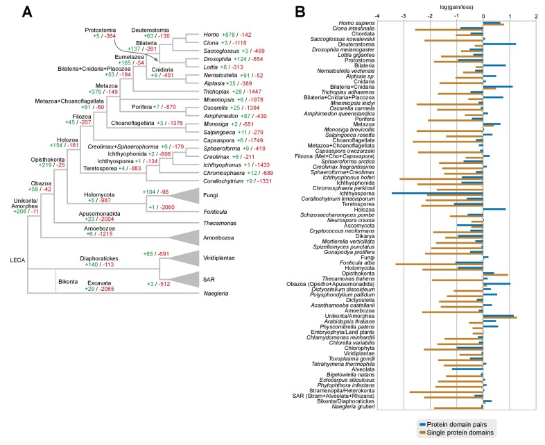
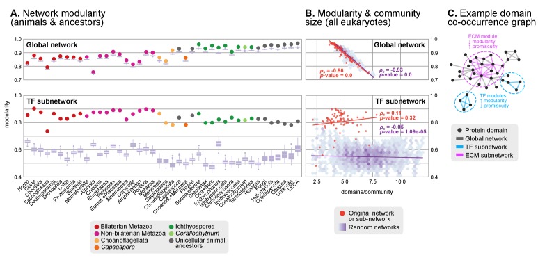
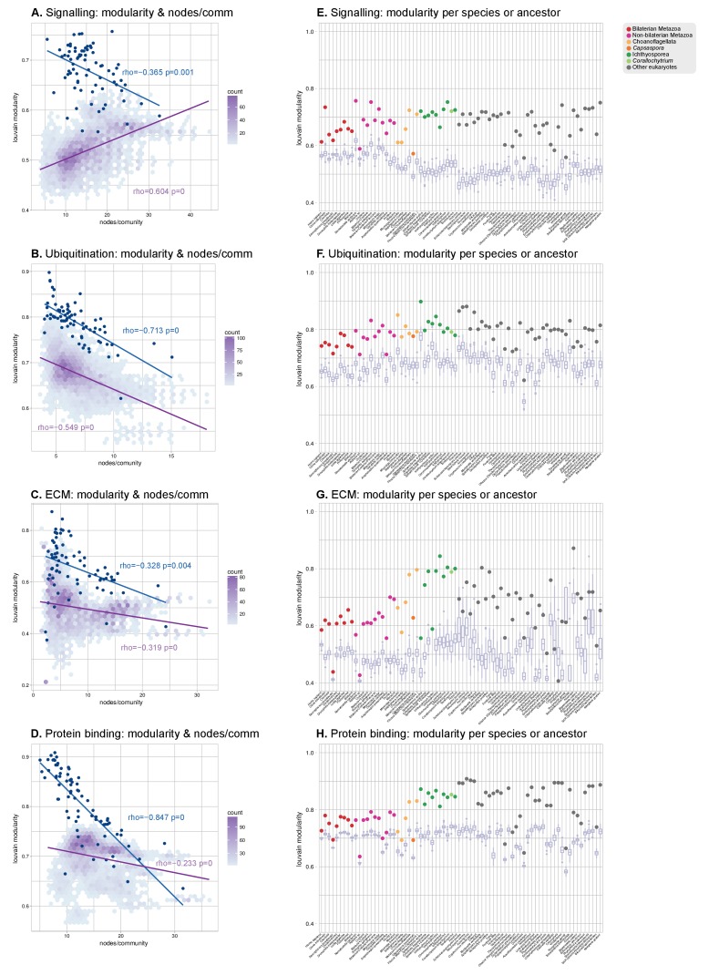
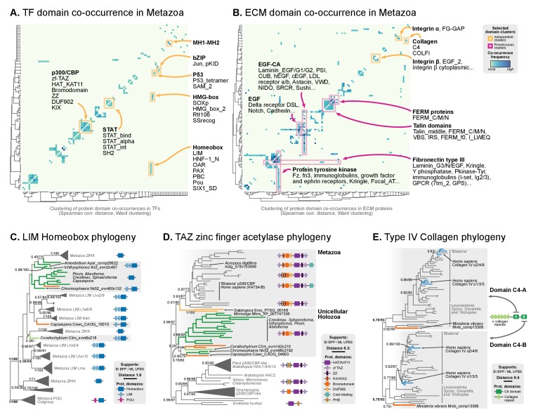
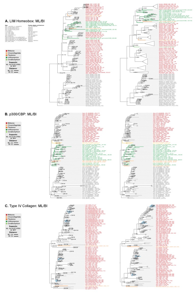
Which genomic innovations underpinned the origin of multicellular animals is still an open debate. Here, we investigate this question by reconstructing the genome architecture and gene family diversity of ancestral premetazoans, aiming to date the emergence of animal-like traits. Our comparative analysis involves genomes from animals and their closest unicellular relatives (the Holozoa), including four new genomes: three Ichthyosporea and Corallochytrium limacisporum. Here, we show that the earliest animals were shaped by dynamic changes in genome architecture before the emergence of multicellularity: an early burst of gene diversity in the ancestor of Holozoa, enriched in transcription factors and cell adhesion machinery, was followed by multiple and differently-timed episodes of synteny disruption, intron gain and genome expansions. Thus, the foundations of animal genome architecture were laid before the origin of complex multicellularity - highlighting the necessity of a unicellular perspective to understand early animal evolution.

Keywords: animal origins; chromosomes; comparative genomics; evolutionary biology; gene family evolution; genes; genomics; holozoans; ichthyosporeans; introns.

Figure 1.. Evolutionary framework and genome statistics of the study.

(A) Schematic phylogenetic tree of eukaryotes, with a focus on the Holozoa. The adjacent table summarizes genome assembly/annotation statistics. Data sources: red asterisks denote Teretosporea genomes reported here; double asterisks denote organisms sequenced for this study; † previously sequenced genomes (King et al., 2008; Fairclough et al., 2013; Suga et al., 2013); ‡ organisms for which transcriptomic data exists but no genome is available (Torruella et al., 2015). (B) Overview of the phenotypic traits of each group of unicellular Holozoa, focusing on their multicellular-like characteristics. For further details, see (Torruella et al., 2015; Mendoza et al., 2002; Marshall et al., 2008; Glockling et al., 2013). Figure 1—source data 1 and 2. DOI: http://dx.doi.org/10.7554/eLife.26036.003

Figure 1—figure supplement 1.. Comparisons of gene length of one-to-one orthologs from pair-wise comparisons of all 10 unicellular Holozoa.

Dots around the diagonal lines indicate that orthologs from both organisms have identical lengths. Note that Abeoforma and Pirum have abundant incomplete orthologous sequences. DOI: http://dx.doi.org/10.7554/eLife.26036.006

Figure 2.. Phylogenomic tree of Unikonta/Amorphea.

Phylogenomic analysis of the BVD57 taxa matrix. Tree topology is the consensus of two Markov chain Monte Carlo chains run for 1231 generations, saving every 20 trees and after a burn-in of 32%. Statistical supports are indicated at each node: (i) non-parametric maximum likelihood ultrafast-bootstrap (UFBS) values obtained from 1000 replicates using IQ-TREE and the LG + R7+C60 model; (ii) Bayesian posterior probabilities (BPP) under the LG+Γ7 + CAT model as implemented in Phylobayes. Nodes with maximum support values (BPP = 1 and UFBS = 100) are indicated by a black bullet. See Figure 2—figure supplement 1 for raw trees with complete statistical supports. Figure 2—source data 1. DOI: http://dx.doi.org/10.7554/eLife.26036.007

Figure 2—figure supplement 1.. Phylogenomic analysis of the BVD57 matrix using (A) IQ-TREE maximum likelihood and the LG + R7+C60 model (supports are SH-like approximate likelihood ratio test/UFBS, respectively); (B) IQ-TREE maximum likelihood and the LG + R7+PMSF model (fast CAT approximation; non-parametric bootstrap supports); and (C) Phylobayes Bayesian inference under the LG+Γ7 + CAT model (BPP supports).

DOI: http://dx.doi.org/10.7554/eLife.26036.009

Figure 3.. Patterns of genome evolution across unicellular Holozoa.

(A) Genome size and composition in terms of coding exonic, intronic and intergenic sequences of unicellular holozoan and selected metazoans. Percentage of repetitive sequences shown as black bars. Genome size of the Metazoa LCA (gray bar) from (Simakov and Kawashima, 2017) (exonic, intronic and intergenic composition not known). (B) Profile of TE composition for selected organisms. Density plots indicate the sequence similarity profile of the TE complement in each organism. Embedded pie-charts denote the relative abundance, in nucleotides, of the main TE superclasses in each genome: retrotransposons (SINE, LINE and LTR), DNA transposons (DNA) and unknown. N_c: total number TE copies in the genome; N_f: number of families to which these belong; P_25f and P_75f: percentage of most-frequent TE families that account for 25% and 75% of the total number of TE copies, respectively. (C) Heatmap of pairwise microsynteny conservation between 10 unicellular holozoan genomes. Species ordered according the number of shared syntenic genes (Euclidean distances, Ward clustering). At the right: selected pairwise comparisons of syntenic single-copy orthologs between unicellular holozoan genomes. Numbers denote number of syntenic genes, total number of single-copy orthologs, and proportions (%) of syntenic genes per the compared orthologs. Circle segments are scaffolds sharing ortholog pairs, connected by gray lines. (D) Phylogenetic distances between unicellular holozoans and four selected animals: Homo sapiens, Nematostella vectensis, Trichoplax adhaerens and Amphimedon queenslandica. Red asterisks denote organisms that have lower phylogenetic distances to metazoans than one (single asterisk) or both choanoflagellates (double asterisks) (p value < 0.05 in Wilcoxon rank sum test). † indicates significantly higher distances between Corallochytrium and metazoans. Figure 1—source data 1, Figure 3—source data 1, 2 and 3. DOI: http://dx.doi.org/10.7554/eLife.26036.010

Figure 3—figure supplement 1.. Profile of TE composition of unicellular Holozoa.

(A-J) Profile of transposable element (TE) composition of 10 unicellular Holozoa, including (i) distribution of sequence similarity frequencies within the TE complement obtained from BLAST alignments (minimum 70% identity and 80 bp alignment length); (ii) same data but using density-normalized plots; and (iii) raw counts of hits for each TE family, indicating the number of families with hits (NFH) for each species. Each third panel illustrates how TE complements can be biased towards a handful of families with a high number of similarity hits (e.g. Monosiga or Pirum) or, conversely, exhibit even distributions (e.g. Corallochytrium). DOI: http://dx.doi.org/10.7554/eLife.26036.014

Figure 3—figure supplement 2.. Shared TEs between unicellular Holozoa and animal genomes.

(A) Pattern of presence/absence of TE families across Holozoa (11 animals and 10 unicellular holozoans). Dendrogram at the left represents the sorting of TE families by Euclidean distance and Ward clustering. Colored column indicates presence in both unicellular and multicellular holozoans (green) or just on unicellular or multicellular holozoans (light brown). (B) List of the most abundant TE families across holozoans, including only most abundant families present in >1 species and accounting for 25% of the copies in a given genome. Complete table in Figure 3—source data 3. (C–E) Distribution of the number of TE families present in unicellular holozoans per number of species (X axis). The color code indicates presence in both unicellular and multicellular holozoans (green) or just on unicellular or multicellular holozoans (light brown). Panel C includes all TE families; panel D only most abundant TEs accounting for 75% of the copies in a given genome (P_75f); panel E id. for 25% of copies (P_25f). DOI: http://dx.doi.org/10.7554/eLife.26036.015

Figure 3—figure supplement 3.. Heatmap of pairwise ratios of ortholog collinearity between 10 unicellular holozoan genomes.

Species are manually ordered by taxonomic classification (no clustering). DOI: http://dx.doi.org/10.7554/eLife.26036.016

Figure 4.. Intron abundance in eukaryotes.

(A) Distribution of intron lengths and number of introns per gene in selected eukaryote genomes. Dots represent median intron lengths and vertical lines delimit the first and third quartiles. Color code denotes taxonomic assignment. Species abbreviation as in Figure 1 and Figure 2—source data 1. (B) Fraction of the genome covered by introns and exons in selected eukaryotes. Dotted line represents the identity between both values. Color code denotes taxonomic assignment. Figure 1—source data 1. DOI: http://dx.doi.org/10.7554/eLife.26036.017

Figure 5.. Intron evolution.

(A) Rates of intron gain and loss per lineage, including extant genomes and ancestral reconstructed nodes. Diameter and color of circles denote the number of introns per kbp of coding sequence at each ancestral node. Bolder edges mark the lines of descent between the LECA and Metazoa/Ichthyophonida, which were characterized by continued high intron densities (see text). Red and green bars represent the inferred number of intron gains (green) and losses (red) in ancestral nodes. (B) Difference between intron site gains and losses in selected ancestors, including animals (left; from Metazoa to Unikonta/Amorphea) and unicellular holozoans (right). For each ancestor, we specify the variance-to-mean ratio of the inferred number of introns from 100 bootstrap replicates (higher values, denoted by lighter purple, indicate less reliable inferences; see Methods. The color code denotes modes of intron evolution: dominance of gains (green), losses (pink) and stasis (light gray). (C) Conservation of the NMD machinery and SR splicing factors in unicellular holozoans (up) and selected ancestors (down). Black dots indicate the presence of an ortholog, and empty dots partial conservation. For the NMD machinery, each column summarizes the presence of multiple gene families (number between brackets). † denotes the ancestral eukaryotic origin of TRA2 according to (Plass et al., 2008). Complete survey at the species and gene levels available as Figure 4—figure supplements 2 and 3. Figure 5—source data 1, 2 and 3. DOI: http://dx.doi.org/10.7554/eLife.26036.018

Figure 5—figure supplement 1.. Classification of intron sites by conservation in protein alignments, as used in (Csűrös and Miklós, 2006; Csurös, 2008).

Grey boxes denote aligned amino acids with gaps (dashed lines). Intron sites (vertical lines) are conserved if they are present in various organisms at the same alignment position and codon phase. The method accounts for loss of intron sites (red crosses), independent gains at the same site (different codon phases), ambiguous sites (in poorly-aligned regions) and unclassifiable sites (non-homologous regions). DOI: http://dx.doi.org/10.7554/eLife.26036.022

Figure 5—figure supplement 2.. Phylogenetic distribution of the NMD machinery, SR splicing factors and RNA-binding domains in eukaryotes.

(A) Phylogenetic distribution of the NMD molecular toolkit across eukaryotes, as defined in Whelan et al. (2015), with a focus on unicellular holozoans and selected metazoans. The analysis includes 12 gene families: the core regulatory factors Upf1, Upf2 and Upf3 (also Smg2-4); the accessory proteins Smg1, Smg5/6/7 and Smg8/9; the release factors eRF1 and eRF3; and the exon junction complex (EJC) proteins eIF4A3, Y14, Magoh and MLN51. Extant species are color-coded by taxonomic assignment. Black dots indicate reconstructed LCAs within the line of descent between Metazoa and the LECA, whereas gray dots indicate LCAs not affiliated with Metaoza. Red, hollow circles indicate that a specific gene is absent from a given animal genome, but nevertheless present in a close relative in the same lineage (e.g., poriferans other than Amphimedon). See Methods for details on ortholog identification. Complete survey at the species level available as Figure 5—source data 3. Note that the core NMD tool-kit is conserved in most post-LECA LCAs, both in the animal and ichthyophonid ancestry. Secondary losses affect extant taxa: Corallochytrium lacks the complete EJC (only eIF4A3 is conserved) and homologs of Smg5/6/7 and Smg8/9. (B) Phylogenetic distribution of the SR splicing factors involved in alternative splicing determination across eukaryotes, as defined in Plass et al. (2008), with a focus on unicellular holozoans and selected metazoans. The analysis is focused on the following RNA-binding genes: SRP20/9G8 (human paralogs SRSF3/7), ASF (human paralogs SRSF1/9), SRP2 (human paralogs SRSF4/5/6), SRP1 (human paralogs SRSF2/8) and TRA2 (human paralogs TRA2A/B). Extant species are color-coded by taxonomic assignment. Black dots indicate reconstructed LCAs within the line of descent between Metazoa and the LECA, whereas gray dots indicate LCAs not affiliated with Metaoza. See Methods for details on ortholog identification. Complete survey at the species level available as Figure 5—source data 3. Note that the complement of SR genes is conserved in most post-LECA LCAs, including Opisthokonta, Holozoa and Metazoa. Secondary losses are, however, frequent in some lineages: SRSF1/9 is lost in Fungi, Teretosporea and Filasterea; Corallochytrium lacks all canonical SR genes but TRA2 and a fragmentary SRSF4/5/6; choanoflagellates have lost SRSF4/5/6, etc. (C) Counts of RNA-binding protein domains in extant eukaryotic genomes. Unicellular holozoans have a rich complement of RNA-binding proteins (domains per species: average 127.8; median 120), albeit less abundant than metazoans’ (domains per species: average 225.3; median 187). DOI: http://dx.doi.org/10.7554/eLife.26036.023

Figure 5—figure supplement 3.. Phylogenetic analysis of (A) eIF4A3, (B) Smg5/6/7, and (C) eRF3, using Maximum likelihood in IQ-TREE (supports are SH-like approximate likelihood ratio test/UFBS, respectively); including Bayesian inference supports for the ortologous groups of interest (BPP statistical supports, in red).

DOI: http://dx.doi.org/10.7554/eLife.26036.024

Figure 6.. Profile of intron site presence across eukaryotes.

(A) Heatmap representing presence/absence of 4312 intron sites (columns) from extant and ancestral holozoan genomes, plus the line of ascent to the LECA (rows). Intron sites and genomes have been grouped according to their respective patterns of co-occurrence (dendrogram based on Spearman correlation distances and Ward clustering algorithm; see Methods). The dendrogram of genome clusterings is shown to the left. Figure 5—source data 2. (B) Phylostratigraphic analysis of the origin of Capsaspora introns, considering all sites (left) and those with putative regulatory sites (right; after [Sebé-Pedrós et al., 2016b]). DOI: http://dx.doi.org/10.7554/eLife.26036.025

Figure 7.. Evolution of protein domain architectures.

(A) Protein domain combination gain and loss per lineage, including extant genomes and ancestral reconstructed nodes. Diameter and color of circles denote the number of different domain combinations (in different gene families) in that node of the tree. Bolder edges mark the line of descent between the LCAs of Opisthokonta and Bilateria, which was generally dominated by gains of protein domain combinations (see text). Red and green bars represent the inferred number of gains and losses, respectively. (B) Gain/loss ratio of protein domain diversity in selected ancestors, including animals (upper chart; from Metazoa to Unikonta/Amorphea) and unicellular holozoans (lower). Heatmap to the right represents the log-ratio value of the diversification rate for selected sub-sets of functionally-related protein domains relevant to multicellularity: green indicates higher-than-average diversification; pink less; white asterisks indicate two-fold or more increases or decreases (all comparisons relative to the whole set of protein domains). Source Data Figure 7—source data 1, 2, 3 and 4. DOI: http://dx.doi.org/10.7554/eLife.26036.026

Figure 7—figure supplement 1.. Gains and losses of individual protein domains across eukaryotes.

(A) Ancestral reconstruction of gains (green) and losses (red) of protein domains per lineage, based on Dollo parsimony. Note that, in contrast with the evolution of protein domain combinations here most nodes are dominated by losses. The most notable exceptions are the Metazoa and Opisthokonta LCAs (dominated by gains) and its unicellular ancestors from Holozoa to Choanoflagellata + Metazoa LCAs (in which gains and losses are in a relative stasis). Figure 7—source data 3. (B) Log-ratio of gains-to-losses for single protein domains (brown bars) and protein domain pairs (blue bars), based on the respective ancestral reconstructions. Positive values thus mean that gains are greater than losses. Loss of single protein domains dominates in most nodes, but gains in protein domain combinations can nevertheless outweigh losses in many ancestors (e.g., Holozoa or Metazoa LCAs). DOI: http://dx.doi.org/10.7554/eLife.26036.031

Figure 8.. Protein domain architecture networks.

(A and B) Modularity and community size of the global network of domain pairs (upper panels) and the TF subnetwork (lower panels), with ≥90% probability. The modularity parameter measures the fraction of the intra-community edges in the network, minus the expected value in a random network (takes values from 0 to 1; see Materials and methods and [Newman and Girvan, 2004]). Panels at the left show the observed modularity of the protein domain (sub)networks of various genomes (Holozoa and selected ancestors; dots are taxa-colored). Purple box plots represent the distribution of simulated modularities from 100 rewirings of the original organism-specific networks, while keeping a constant vertex degree distribution. Panels to the right show the relationship between modularities and the number of domains/community, both for actual genomes (orange) and simulated rewired networks (purple density plot, see Methods). Monotonic dependence between modularity and domains/community was tested for each set of data (global, TF and their respective simulations) using Spearman's rank correlation coefficient (ρ_s), and linear regression fits are included for clarity. Note that simulated TF subnetworks are less modular and have more domains/community than the original ones, signaling their higher-than-expected modularities. Note that the scales of the vertical axes change between upper and lower panels. (C) Example of protein domain co-occurrence network. Vertices represent domains, linked by edges if they co-occur within the same gene family. Two subnetworks are highlighted in yellow (domain pairs occurring in TF genes) or green (same for signaling genes). Figure 7—source data 1 and 2, Figure 1—source data 2. DOI: http://dx.doi.org/10.7554/eLife.26036.032

Figure 8—figure supplement 1.. Modularity of protein domain co-occurrence networks of multicellularity-related gene sets across eukaryotes.

(A–D) Modularity and community size of the functional sub-networks based on domains related to signaling (Richter and King, 2013), ubiquitination (Grau-Bové et al., 2015), ECM (Richter and King, 2013; Sebé-Pedrós et al., 2010; Hynes, 2012) and protein binding (Mitchell et al., 2015) functions. Blue dots indicate real genomes, and the purple density plot indicates the values of the simulated rewired networks. Monotonic dependence between modularity and domains/community was tested for each set of data using Spearman's rank correlation coefficient (ρ_s); linear regression fits are included for clarity. All sub-networks (A–D) have the same decreasing trend as the global sub-network of Figure 8A–B, and contrast with the results for TFs. (E–H) Modularity of the functional sub-network based on domains related to signaling, ubiquitination, ECM and protein binding functions (same domains as in A-D), per species or ancestral node (colored dots). Purple box plots represent the distribution of simulated modularities from 100 rewirings of the original organism-specific networks, while keeping a constant vertex degree distribution. Note the decreased modularities shown by metazoans (red and pink) in all sub-networks. DOI: http://dx.doi.org/10.7554/eLife.26036.033

Figure 9.. Phylogenetic analysis of the premetazoan gene families LIM Homeobox, CBP/p300 and type IV collagen.

(A and B) Protein domain co-occurrence matrices of transcription factor (TF) (A) or extracellular matrix (ECM)-related gene families (B), inferred at the LCA of Metazoa (≥90% probability). Horizontal and vertical axes of the heatmap represent individual protein domains and their mutual co-occurrence frequency, and have been clustered according to the number of shared domains (dendrogram based on Spearman correlation distances and Ward clustering algorithm). Note that, for TFs, most co-occurrence clusters are located along the diagonal, indicating isolated domain communities; whereas ECM genes tend to contain promiscuous domains shared in multiple domain co-occurrence communities. Representative examples of independent and promiscuous domain clusters have been highlighted in both heat maps (orange and pink, respectively). (C) Phylogenetic tree of LIM Homeobox TFs, with mapped protein domains architectures. (D) Phylogenetic tree of CBP/p300 TFs based on HAT/KAT11 domain, with mapped consensus protein domain architectures. (E) Phylogeny of type IV collagen genes based on the C4 domain. All extant homologs, from Ministeria to animals, have a C4-C4 dual arrangement of filozoan origin (reflected in the phylogeny by two parallel clades representing the first and second domains within each gene). Ministeria (orange) and human (blue) homologs are highlighted. In C, D and E panels, bold branches represent unicellular holozoan genes and are color-coded by taxonomic assignment. All trees are Bayesian inferences (BI). Protein domain architectures and statistical supports (BPP/UFBS) are shown for selected nodes (see Figure 9—figure supplement 1 for the complete BI and ML trees with statistical supports). Figure 7—source data 1 and 2. DOI: http://dx.doi.org/10.7554/eLife.26036.034

Figure 9—figure supplement 1.. Phylogenetic analysis of the (A) LIM-Homeobox, (B) p300/CBP, and (C) Collagen Type IV, using Maximum likelihood in IQ-TREE (supports are SH-like approximate likelihood ratio test/UFBS, respectively) and Bayesian inference in Mr. Bayes (BPP statistical supports).

DOI: http://dx.doi.org/10.7554/eLife.26036.035

Figure 10.. Domain combinations that appear in transcription factor (TF) families in unicellular premetazoans, from the LCA of Unikonta/Amorphea to the LCA of Metazoa.

First and second columns indicate the TF family and its inferred evolutionary origin, respectively (from [de Mendoza et al., 2013]). Subsequent columns list (i) the p-value of a Fisher's exact test for the relative enrichment of that TF family in that node of the tree (compared to other domains that rearrange there; p-values<0.05 in green); and (ii) the accessory domains that appear within each TF family. Figure 7—source data 2, Table 1. DOI: http://dx.doi.org/10.7554/eLife.26036.036

References

1. Abedin M, King N. The premetazoan ancestry of cadherins. Science. 2008;319:946–948. doi: 10.1126/science.1151084. - DOI - PubMed
1. Andrews S. FastQC. [3 May, 2016];2014 http://www.bioinformatics.bbsrc.ac.uk/projects/fastqc
1. Aouacheria A, Geourjon C, Aghajari N, Navratil V, Deléage G, Lethias C, Exposito JY. Insights into early extracellular matrix evolution: spongin short chain collagen-related proteins are homologous to basement membrane type IV collagens and form a novel family widely distributed in invertebrates. Molecular Biology and Evolution. 2006;23:2288–2302. doi: 10.1093/molbev/msl100. - DOI - PubMed
1. Bao W, Kojima KK, Kohany O. Repbase Update, a database of repetitive elements in eukaryotic genomes. Mobile DNA. 2015;6:4–9. doi: 10.1186/s13100-015-0041-9. - DOI - PMC - PubMed
1. Barbosa-Morais NL, Irimia M, Pan Q, Xiong HY, Gueroussov S, Lee LJ, Slobodeniuc V, Kutter C, Watt S, Colak R, Kim T, Misquitta-Ali CM, Wilson MD, Kim PM, Odom DT, Frey BJ, Blencowe BJ. The evolutionary landscape of alternative splicing in vertebrate species. Science. 2012;338:1587–1593. doi: 10.1126/science.1230612. - DOI - PubMed
Publication types