. 2016:29:1369-1377.

Deep Learning Models of the Retinal Response to Natural Scenes

Affiliations

Deep Learning Models of the Retinal Response to Natural Scenes

Lane T McIntosh et al. Adv Neural Inf Process Syst. 2016.

Abstract

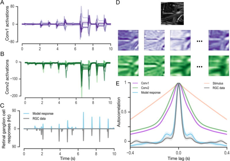
A central challenge in sensory neuroscience is to understand neural computations and circuit mechanisms that underlie the encoding of ethologically relevant, natural stimuli. In multilayered neural circuits, nonlinear processes such as synaptic transmission and spiking dynamics present a significant obstacle to the creation of accurate computational models of responses to natural stimuli. Here we demonstrate that deep convolutional neural networks (CNNs) capture retinal responses to natural scenes nearly to within the variability of a cell's response, and are markedly more accurate than linear-nonlinear (LN) models and Generalized Linear Models (GLMs). Moreover, we find two additional surprising properties of CNNs: they are less susceptible to overfitting than their LN counterparts when trained on small amounts of data, and generalize better when tested on stimuli drawn from a different distribution (e.g. between natural scenes and white noise). An examination of the learned CNNs reveals several properties. First, a richer set of feature maps is necessary for predicting the responses to natural scenes compared to white noise. Second, temporally precise responses to slowly varying inputs originate from feedforward inhibition, similar to known retinal mechanisms. Third, the injection of latent noise sources in intermediate layers enables our model to capture the sub-Poisson spiking variability observed in retinal ganglion cells. Fourth, augmenting our CNNs with recurrent lateral connections enables them to capture contrast adaptation as an emergent property of accurately describing retinal responses to natural scenes. These methods can be readily generalized to other sensory modalities and stimulus ensembles. Overall, this work demonstrates that CNNs not only accurately capture sensory circuit responses to natural scenes, but also can yield information about the circuit's internal structure and function.


Figures

Figure 1
Figure 1
A schematic of the model architecture. The stimulus was convolved with 8 learned spatiotemporal filters whose activations were rectified. The second convolutional layer then projected the activity of these subunits through spatial filters onto 16 subunit types, whose activity was linearly combined and passed through a final soft rectifying nonlinearity to yield the predicted response.
Figure 2
Figure 2
Model performance. (A,B) Correlation coefficients between the data and CNN, GLM or LN models for white noise and natural scenes. Dotted line indicates a measure of retinal reliability (See Methods). (C) Receiver Operating Characteristic (ROC) curve for spike events for CNN, GLM and LN models. (D) Spike rasters of one example retinal ganglion cell responding to 6 repeated trials of the same randomly selected segment of the natural scenes stimulus (black) compared to the predictions of the LN (red), GLM (green), or CNN (blue) model with Poisson spike generation used to generate model rasters. (E) Peristimulus time histogram (PSTH) of the spike rasters in (D).
Figure 3
Figure 3
Model parameters visualized by computing a response-weighted average for different model units, computed for models trained on spatiotemporal white noise stimuli (left) or natural image sequences (right). Top panel (purple box): visualization of units in the first layer. Each 3D spatiotemporal receptive field is displayed via a rank-one decomposition consisting of a spatial filter (top) and temporal kernel (black traces, bottom). Bottom panel (green box): receptive fields for the second layer units, again visualized using a rank-one decomposition. Natural scenes models required more active second layer units, displaying a greater diversity of spatiotemporal features. Receptive fields are cropped to the region of space where the subunits have non-zero sensitivity.
Figure 4
Figure 4
CNNs overfit less and generalize better across stimulus class as compared to simpler models. (A) Held-out performance curves for CNN (~150,000 parameters) and GLM/LN models cropped around the cell’s receptive field (~4,000 parameters) as a function of the amount of training data. (B) Correlation coefficients between responses to natural scenes and models trained on white noise but tested on natural scenes. See text for discussion.
Figure 5
Figure 5
Training with added noise recovers retinal sub-Poisson noise scaling property. (A) Variance versus mean spike count for CNNs with various strengths of injected noise (from 0.1 to 10 standard deviations), as compared to retinal data (black) and a Poisson distribution (dotted red). (B) The same plot as A but with each curve normalized by the maximum variance. (C) Variance versus mean spike count for CNN models with noise injection at test time but not during training.
Figure 6
Figure 6
Visualizing the internal activity of a CNN in response to a natural scene stimulus. (A–C) Time series of the CNN activity (averaged over space) for the first convolutional layer (8 units, A), the second convolutional layer (16 units, B), and the final predicted response for an example cell (C, cyan trace). The recorded (true) response is shown below the model prediction (C, gray trace) for comparison. (D) Spatial activation of example CNN filters at a particular time point. The selected stimulus frame (top, grayscale) is represented by parallel pathways encoding spatial information in the first (purple) and second (green) convolutional layers (a subset of the activation maps is shown for brevity). (E) Autocorrelation of the temporal activity in (A–C). The correlation in the recorded firing rates is shown in gray.
Figure 7
Figure 7
Recurrent neural network (RNN) layers capture response features occurring over multiple seconds. (A) A schematic of how the architecture from Figure 2.1 was modified to incorporate the RNN at the last layer of the CNN. (B) Response of an RNN trained on natural scenes, showing a slowly adapting firing rate in response to a step change in contrast.

References

    1. Gollisch Tim, Meister Markus. Eye smarter than scientists believed: neural computations in circuits of the retina. Neuron. 2010;65(2):150–164. - PMC - PubMed
    1. Pillow Jonathan W, Shlens Jonathon, Paninski Liam, Sher Alexander, Litke Alan M, Chichilnisky EJ, Simoncelli Eero P. Spatio-temporal correlations and visual signalling in a complete neuronal population. Nature. 2008;454(7207):995–999. - PMC - PubMed
    1. Rust Nicole C, Schwartz Odelia, Movshon J Anthony, Simoncelli Eero P. Spatiotemporal elements of macaque v1 receptive fields. Neuron. 2005;46(6):945–956. - PubMed
    1. Kastner David B, Baccus Stephen A. Coordinated dynamic encoding in the retina using opposing forms of plasticity. Nature neuroscience. 2011;14(10):1317–1322. - PMC - PubMed
    1. Baccus Stephen A, Meister Markus. Fast and slow contrast adaptation in retinal circuitry. Neuron. 2002;36(5):909–919. - PubMed

LinkOut - more resources