Effect of Interactions between Harvester Ants on Forager Decisions

Abstract

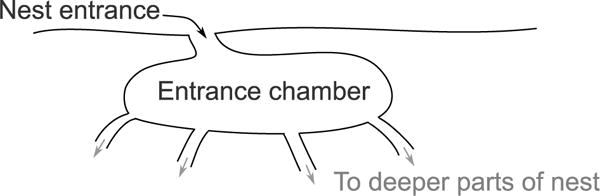
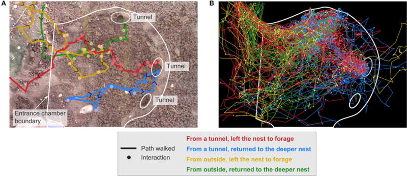
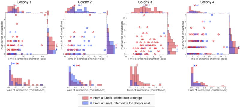
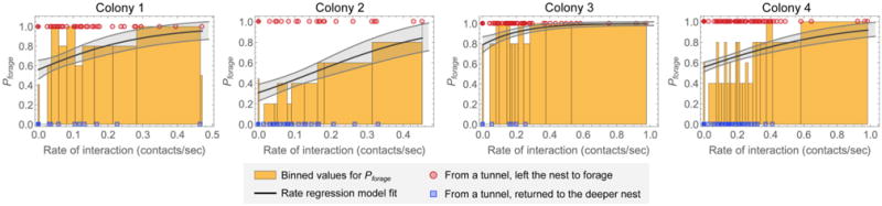
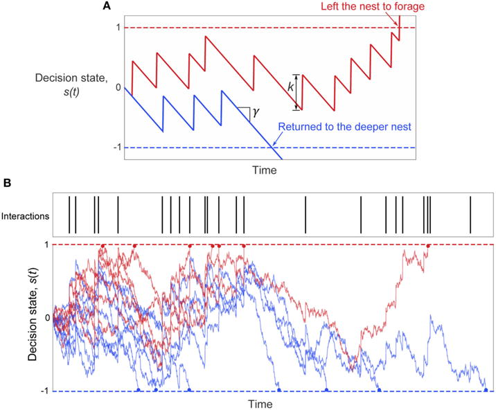
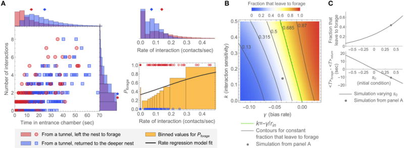
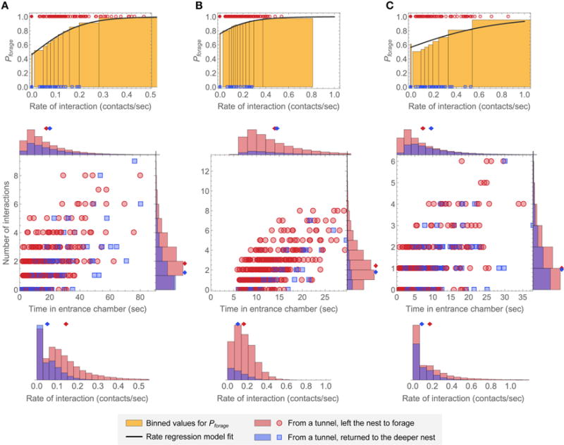
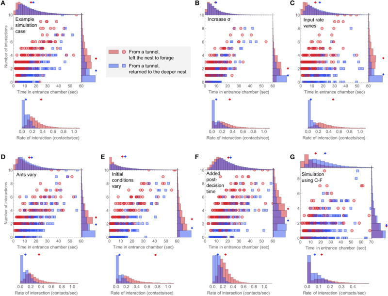
Harvester ant colonies adjust their foraging activity to day-to-day changes in food availability and hour-to-hour changes in environmental conditions. This collective behavior is regulated through interactions, in the form of brief antennal contacts, between outgoing foragers and returning foragers with food. Here we consider how an ant, waiting in the entrance chamber just inside the nest entrance, uses its accumulated experience of interactions to decide whether to leave the nest to forage. Using videos of field observations, we tracked the interactions and foraging decisions of ants in the entrance chamber. Outgoing foragers tended to interact with returning foragers at higher rates than ants that returned to the deeper nest and did not forage. To provide a mechanistic framework for interpreting these results, we develop a decision model in which ants make decisions based upon a noisy accumulation of individual contacts with returning foragers. The model can reproduce core trends and realistic distributions for individual ant interaction statistics, and suggests possible mechanisms by which foraging activity may be regulated at an individual ant level.

Keywords: collective behavior; decision-making; integrator; sequential sampling model; stochastic accumulator.

FIGURE 1. Structure of a typical entrance chamber

Schematic shows a cross-sectional view of an entrance chamber. Potential forager ants interact in the entrance chamber before deciding whether to leave the nest to forage or return to a tunnel leading to a deeper part of the nest. A typical entrance chamber is 5–10 cm wide.

FIGURE 2. Trajectories of returning and potential foragers, grouped by start location and end action

A potential forager comes from a tunnel into the entrance chamber and either leaves the nest to forage (red) or returns to the deeper nest (blue). A returning forager comes into the entrance chamber from outside the nest and either leaves the nest to forage (yellow) or returns to the deeper nest (green). This example from colony 1 shows: (A) One ant in each category, and (B) All tracked ants in each category.

FIGURE 3. Number of interactions, time in the entrance chamber, and rate of interaction of potential foragers

For each of the observations of a colony (columns), plots show the number of interactions and time spent in the entrance chamber for potential foragers from a tunnel that left the nest to forage (red points) or returned to the deeper nest (blue points). Histograms show the corresponding distributions for number of interactions, time in the entrance chamber, and rate of interaction. The per-ant mean and standard error of the mean for each quantity are displayed on each histogram.

FIGURE 4. Rate regression fit for fraction that leave the nest to forage as a function of interaction rate

Results are shown for each observation of a colony. Red points show interaction rates of ants that left the nest to forage, and blue points show interaction rates of ants that returned to the deeper nest. The bins for P_forage are determined by sorting the nonzero interaction rates, forming bins with a fixed number of points per bin (5 points per bin was used), and calculating the fraction of points in each bin that represent ants that left the nest to forage. A separate bin was used for ants with zero interactions; this bin is shown as the separate line at zero. The solid line is a fit of the rate regression model (Equation 1). The fit standard deviation for this model was estimated using bootstrapping; the shaded area around the best fit indicates the standard deviation of the fits for P_forage for each value of the rate of interaction.

FIGURE 5. The two-choice model of ant foraging decisions

(A) Illustration of the decision model parameters. Noise Is omitted to better Illustrate the roles of the parameters γ and k (see Equation 2) in determining the ant’s decision in response to interactions. The bias rate γ sets the mean rate of change of the decision state in the absence of interactions, and k sets the increase in the decision state with each interaction. The initial decision state is set by the parameter s₀, and is set to zero for this example. (B) Example trajectories of the decision state with noise for the set of interaction times shown. Red lines: decision state s(t) of simulated ants that left the nest to forage. Blue lines: decision state s(t) of simulated ants that returned to the deeper nest. The decision time is shown by the dot at the end of each simulated decision path.

FIGURE 6. Representative simulated distributions and model parameter dependence

(A) Simulated distributions of N, T, and r, and rate regression model fit of P_forage to the simulated data. Plots were generated in the same manner as for the data of Figures 3, 4. Parameters for this example were chosen so that the simulations resemble the observation of colony 2: k = 0.14, γ = −0.038, s₀ = 0.39, and σ = 0.21. The mean input interaction rate, r_in = 0.083, was calculated from the data for this observation (see Figure S2). The 2D plot and corresponding N, T, and r distributions display data for 400 simulated ants. The plot of P_forage (bottom right) shows rates as points for 200 simulated ants. (B,C) Effects of changing parameters around the values used in this example. (B) Dependence of the fraction of simulated ants leaving the nest to forage on the interaction sensitivity k and bias rate γ. Parameter values for s₀, σ, and r_in were the same as in (A). The point shows the result from (A), the dashed line shows the “constant decision fraction” line for k = −γ/r_in, and the solid lines show evenly spaced contours at and around the line k = −γ/r_in. (C) Model dependence on the initial decision state s₀. (top) Fraction that leave the nest to forage. (bottom) Difference in average decision time between groups of ants, 〈T_forage〉 − 〈T_return〉, where 〈T_forage〉 is the average decision time for ants that left the nest to forage and 〈T_return〉 is the average decision time for ants that returned to the deeper nest. The point on each plot shows the result from (A). Parameter values for k, γ, σ, and r_in were the same as in (A).

FIGURE 7. Simulated model distributions representative of other colony observations

The parameters in (A–C) were chosen so that the simulated distributions resemble the observations of colonies 1, 3, and 4, respectively. The top row shows binned plots for P_forage as a function of interaction rate in the same manner as Figure 4. The solid lines are fits of the rate regression model to each set of simulated data, and 200 points are shown on each plot for illustration. The bottom row shows 2D plots and corresponding N, T, and r distributions for 400 simulated ants as in Figure 3. (A) k = 0.26, γ = −0.007, s₀ = 0.06, and σ = 0.22, with r_in = 0.083 taken from the data for the observation of colony 1 (Figure S2). (B) k = 0.15, γ = 0.044, S₀ = 0.02, and σ = 0.30. To produce results resembling the time distributions for the observation of colony 3 (Figure 3), a constant post-decision time without interactions of 5 s. was added to each simulated ant. A value of r_in = 0.25 was used to match the overall input rate of interaction for this observation when the added post-decision time is included. (C) k = 0.17, γ = −0.012, S₀ = 0.21, and σ = 0.35, with r_in = 0.117 taken from the data for the observation of colony 4 (Figure S2).

FIGURE 8. Simulating sources of variability

For each case, the number of interactions vs. time in the entrance chamber is plotted for 400 simulated ants, and histograms for the distributions of number of interactions, time in the entrance chamber, and rate of interaction are shown for simulated ants in each group. (A) An example simulation using parameters k = 0.4, γ = −0.06, s₀ = 0, σ = 0.2, and r_in = 0.15. (B–F) show perturbations to this case. (B) Increased noise in the decision variable, from σ = 0.2 to σ = 0.3. (C) The input Poisson interaction rate r_in was drawn from a uniform distribution from 0 to $r_{in}^{\mathit{max}}=0.3$ for each simulated ant. (D) The interaction sensitivity k and bias rate γ were drawn from normal distributions with mean values the same as in panel A, and standard deviations of 50% of the mean. (E) The initial decision state, s₀, was drawn from a uniform distribution from −0.75 to 0.75. (F) Simulated ants have an added post-decision time drawn from a uniform distribution of 0–10 s., during which they continue to engage in interactions at the Poisson rate of r_in = 0.15. (G) An example simulation including all of the added simulation mechanisms shown in (C–F), with parameters chosen to resemble the observation of colony 2. The noise level is σ = 0.21, the input rate of interaction was drawn from a uniform distribution from 0 to $r_{in}^{\mathit{max}}=0.16$, the interaction sensitivity and bias rate were drawn from normal distributions defined by k = 0.14 ± 50% and γ = −0.038 ± 50%, the initial decision state was drawn from a uniform distribution from −0.2 to 0.8, and each simulated ant has an added post-decision time drawn from a uniform distribution from 0 to 5 s, during which it continues to make interactions at a Poisson rate drawn from a uniform distribution from 0 to $r_{in}^{\mathit{max}}=0.16$.

FIGURE 9. Changes in the fraction of ants that leave the nest to forage with mean input interaction rate

Shown are simulation results for the fraction of ants that leave the nest to forage as a function of the mean input interaction rate r_in (solid lines). These were obtained by performing multiple simulations with different values of r_ln, while other parameters remained the same. Rate regression fits for P_forage(r), reproduced from Figures 6A, 7, are shown for comparison; note that these simulations had fixed r_in values and the different values of r shown here result from Poisson variability across ants in the experienced rate of interactions (number of contacts per second). Parameter sets 1, 2, 3, and 4 were taken from Figures 6A, 7A–C, to resemble the observations for colonies 1, 2, 3, and 4, respectively. Note that much of the difference between the curves for parameter set 3 is due to the added 5 s post-decision time in the simulations of Figure 7B, which was not included when generating the fraction that leave to forage as a function of r_in.

FIGURE 10. Possible mechanisms underlying regulation of foraging rate

The fraction that leave the nest to forage f (shown decreasing progressively from the left column to the right column) depends on the interaction sensitivity k and constant bias rate γ. Individual panels show the interaction rate distributions for simulated ants that left the nest to forage vs. those that returned to the deeper nest. Parameter values of S₀, σ, and r_in were used from Figure 6A, and the evidence parameters k and γ were given the following values: (left-top) k = 0.36, γ = −0.038, (left-bottom) k = 0.22, γ = −0.023, (middle) k = 0.22, γ = −0.038, (right-top) k = 0.026, γ = −0.038, (right-bottom) k = 0.22, γ = −0.056.

References

1. Beverly BD, McLendon H, Nacu S, Holmes S, Gordon DM. How site fidelity leads to individual differences in the foraging activity of harvester ants. Behav Ecol. 2009;20:633–638. doi: 10.1093/beheco/arp041. - DOI
1. Bogacz R, Brown E, Moehlis J, Holmes P, Cohen JD. The physics of optimal decision making: a formal analysis of models of performance in two-alternative forced-choice tasks. Psychol Rev. 2006;113:700–765. doi: 10.1037/0033-295X.113.4.700. - DOI - PubMed
1. Brunton BW, Botvinick MM, Brody CD. Rats and humans can optimally accumulate evidence for decision-making. Science. 2013;340:95–98. doi: 10.1126/science.1233912. - DOI - PubMed
1. Burd M, Shiwakoti N, Sarvi M, Rose G. Nest architecture and traffic flow: large potential effects from small structural features. Ecol Entomol. 2010;35:464–468. doi: 10.1111/j.1365-2311.2010.01202.x. - DOI
1. Busemeyer JR, Townsend JT. Decision field theory: a dynamic-cognitive approach to decision making in an uncertain environment. Psychol Rev. 1993;100:432–459. doi: 10.1037/0033-295X.100.3.432. - DOI - PubMed