Superresolution expansion microscopy reveals the three-dimensional organization of the Drosophila synaptonemal complex

Abstract

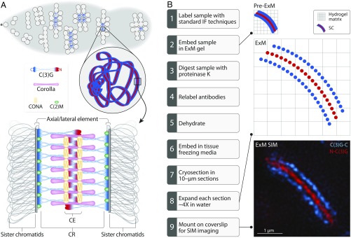
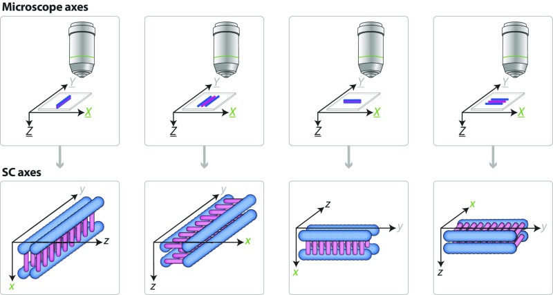
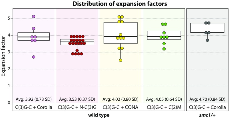
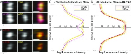
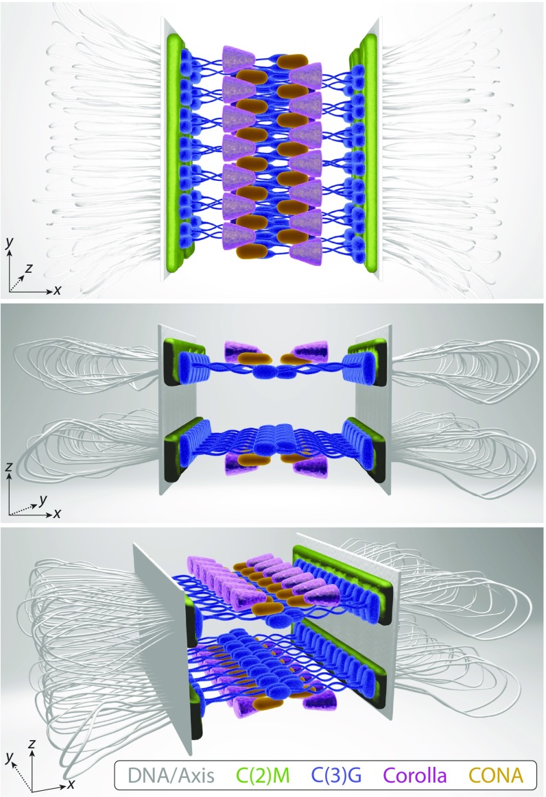
The synaptonemal complex (SC), a structure highly conserved from yeast to mammals, assembles between homologous chromosomes and is essential for accurate chromosome segregation at the first meiotic division. In Drosophila melanogaster, many SC components and their general positions within the complex have been dissected through a combination of genetic analyses, superresolution microscopy, and electron microscopy. Although these studies provide a 2D understanding of SC structure in Drosophila, the inability to optically resolve the minute distances between proteins in the complex has precluded its 3D characterization. A recently described technology termed expansion microscopy (ExM) uniformly increases the size of a biological sample, thereby circumventing the limits of optical resolution. By adapting the ExM protocol to render it compatible with structured illumination microscopy, we can examine the 3D organization of several known Drosophila SC components. These data provide evidence that two layers of SC are assembled. We further speculate that each SC layer may connect two nonsister chromatids, and present a 3D model of the Drosophila SC based on these findings.

Keywords: expansion microscopy; meiosis; sister chromatids; structured illumination microscopy; synaptonemal complex.

Fig. 1.

Drosophila SC biology and expansion protocol. (A) At the anterior tip (asterisk) of the germarium, a cystoblast undergoes four incomplete mitotic divisions to produce a 16-cell interconnected cyst. Euchromatic SC assembly begins in these 16-cell cysts and quickly reaches full length in up to four nuclei within each cyst. At the posterior end of the germarium, only one nucleus in the cyst retains full-length SC. Previous studies demonstrated that C(2)M (green) localizes in the LE; C(3)G homodimers interact to span the CR of the SC, with the C termini of C(3)G (blue) localizing to the LEs and the N termini (red) localizing in the CE; Corolla (pink) lies in the CR; and CONA (yellow) localizes to the CE (reviewed in ref. 1). (B) To adapt ExM to SIM, samples must be prepared and sectioned as shown. The image shows the C (blue) and N (red) termini of C(3)G.

Fig. 2.

ExM SIM images of approximately fourfold-expanded SC showing partial z projections of the SC-containing nuclei labeled for C(3)G-C (blue) and one of C(2)M (green), Corolla (pink), CONA (yellow), or N-C(3)G (red). Dashed boxes designate the region of the image shown in the zoomed-in view, arrows indicate regions in which splitting of the protein is observed in x, and arrowheads indicate regions in which splitting of the protein is observed in z. (Scale bars represent expanded distances.)

Fig. S1.

Diagram of the microscope and the SC axes. The X, Y, and Z axes of the microscope correspond to the width (X) and length (Y) of the stage and the vertical movement of the stage during 3D image stack acquisition (Z). The x, y, and z axes of the SC correspond to the width (x), length (y), and depth (z) of the SC. Diagrammed are the various rotations that the SC can undergo with the appropriate axes labeled on top of the SC. Note that the microscope dimensions never change position, only the SC dimensions change as the SC rotates. Blue represents the LE of the SC, and pink represents the CR of the SC.

Fig. S2.

STED image of unexpanded SC labeling the C(3)G C termini (blue) and Corolla (pink). Regions a and b are two areas in which the SC has turned on its side, showing that Corolla is splitting in z. Dashed boxes designate the region of the image shown in the zoomed-in view, and arrowheads indicate regions where Corolla splitting is observed.

Fig. 3.

Analysis of average x and z profiles of SC proteins. (A) Image analysis workflow. Segments were traced of either flat SC with two clearly observable C(3)G-C tracks (type 1 SC) or turned SC where two C(3)G-C tracks were no longer distinguishable (type 2 SC). In type 1 SC, the microscope axes (XYZ) match the SC axes (xyz); however, in type 2 SC, the SC is turned on its side, placing the SC x-axis along the Z-axis of the microscope and the SC z-axis into the XY microscope plane. Using ImageJ, segments were straightened in 3D along the y-axis of the SC and each slice was then projected along the y-axis to create the average z profile. For type 2 SC, images were rotated to position the x-axis of the SC on the bottom for ease of viewing. Line profiles were drawn on the averaged xz images along either the x-axis (type 1 SC) or the z-axis (type 2 SC), as shown. Then line profiles were averaged together to plot the average distribution of fluorescence intensity. (Scale bars: expanded distances, 250 nm.) (B and C) Representative averaged xz images for type 1 SC (B) and type 2 SC (C) labeled for C(3)G-C (blue), Corolla (pink), CONA (yellow), N-C(3)G (red), and C(2)M (green). The variation observed in these images reflects the distortion from the microscope Z-axis; for a perfect image, the SC must lie completely flat with its side to the microscope, but type 2 SC frequently turns and twists and thus shows more variability than type 1 images. (Scale bars: expanded distances, 250 nm.) (D and E) Multiple line profiles along the x-axis [D: N-C(3)G, n = 21 SC fragments from 8 nuclei; C(3)G-C, n = 21 SC fragments from 8 nuclei; Corolla, n = 7 SC fragments from 6 nuclei; CONA, n = 9 SC fragments from 7 nuclei; C(2)M, n = 9 SC fragments from 4 nuclei] or z-axis [E: N-C(3)G, n = 15 SC fragments from 8 nuclei; C(3)G-C, n = 10 SC fragments from 8 nuclei; Corolla, n = 12 SC fragments from 6 nuclei; CONA, n = 12 SC fragments from 7 nuclei; C(2)M, n = 15 SC fragments from 4 nuclei] were averaged together and then mirrored to generate the distribution of the SC components along the axes. Error bars indicate SE. For both distributions, an expansion factor correction was applied (Materials and Methods) to determine the approximate unexpanded distances in nm. (F) Modeled positions of C(3)G-C (blue), Corolla (pink), CONA (yellow), N-C(3)G (red), and C(2)M (green) based on the line profiles in D and E. (Scale bar: biological distance, 50 nm.)

Fig. S3.

Boxplots displaying the expansion factor values for each dataset analyzed in Fig. 3 and Fig. S4. Average expansion factors and SDs are shown at the bottom of each plot.

Fig. S4.

ExM SIM in an SMC1 deficiency heterozygote (smc1/+). (A) SIM images of WT SC (Top) and smc1/+ SC (Bottom) labeling the C(3)G C termini (blue) and Corolla (pink). (B) The average distribution along the z-axis from ExM SIM images of WT and smc1/+. The analysis was performed as described in Fig. 3. WT: n = 12 SC fragments from six nuclei; smc1/+: n = 12 SC fragments from four nuclei.

Fig. 4.

Relative positions of CONA, Corolla, and N-C(3)G. (A) Representative averaged xz images of Corolla (pink) and CONA (yellow). (B) Representative averaged xz images of N-C(3)G (red) and CONA (yellow). (C) Multiple line profiles along the z-axis were averaged together and then mirrored to generate the z distribution of Corolla (n = 10 SC fragments from 3 nuclei) and CONA (n = 9 SC fragments from 3 nuclei). (D) Multiple line profiles along the z-axis were averaged together and then mirrored to generate the z distribution of CONA (n = 11 SC fragments from 5 nuclei) and N-C(3)G (n = 10 SC fragments from 5 nuclei). An expansion factor correction could not be applied to these samples (Materials and Methods); therefore, the relative distance is in pixel units. Error bars indicate SE. (Scale bars: expanded distances, 250 nm.)

Fig. S5.

Analysis of the distribution of Corolla in xy. (A) Averaged xz images of C(3)G C termini (blue) and Corolla (pink) from type 1 SC. (Scale bars represent expanded distances.) (B) Immuno-EM image of Corolla labeled with gold particles. Arrowheads mark the positions of the gold particles. (C) Histogram of the distribution of Corolla gold particles (n = 51) based on immuno-EM. Overlaid on the histogram is the average intensity of the SC to illustrate the locations of the LEs in relation to the position of the Corolla gold particles. This average intensity is determined by drawing a line profile across the SC in the EM images and then measuring the intensity of the image across that line. These intensity measurements are then averaged together to give the average intensity of the SC.

Fig. S6.

ExM SIM of CONA-Venus. (A and B) Representative partial z projection images of type 1 SC segments from flies expressing CONA-Venus under the Nanos Gal4 driver with C(3)G C termini (blue) and CONA-Venus (yellow). Arrowheads indicate regions were CONA-Venus is splitting in xy. (A′) Averaged xz images of C(3)G C termini (blue) and CONA-Venus (yellow) from the type 1 SC segment in A. (Scale bar: expanded distance, 250 nm.) (B′) Averaged xz images of C(3)G C termini (blue) and CONA-Venus (yellow) from the type 1 SC segment in B. (Scale bar: expanded distance, 250 nm.)

Fig. 5.

A 3D model of the Drosophila SC showing two mirrored SC layers in z, each connecting one sister chromatid of each homologous chromosome. C(2)M (green), Corolla (pink), and CONA (yellow) assemble in two tracks in xy, and C(3)G (blue) spans the distance between homologs. Although Corolla and CONA are known to interact and C(2)M is suspected to interact with the C termini of C(3)G, these interactions have yet to be mapped. Chromosome axis proteins (gray) were not directly examined in this study. [Illustration by Ryan Kramer (artist).]

Fig. S7.

Spinning-disk confocal images of expanded SC in which antibodies were added predigestion and/or postdigestion. All of the antibody conditions were imaged on the same day with the same exposure time and laser power, illustrating that the predigestion and postdigestion labeling has the strongest fluorescent signal. The DNA stain DAPI was used to determine the location of the nuclei within each image. (Scale bars: 5 µm.) (A) Only predigestion labeling of C(3)G-C and Corolla with primary and secondary antibodies. (B) Predigestion labeling of C(3)G-C and Corolla with primary antibodies and postdigestion labeling of secondary antibodies. (C) Only postdigestion labeling of C(3)G-C and Corolla with primary and secondary antibodies. (D) Predigestion and postdigestion labeling of C(3)G-C and Corolla with primary and secondary antibodies.

References

1. Cahoon CK, Hawley RS. Regulating the construction and demolition of the synaptonemal complex. Nat Struct Mol Biol. 2016;23:369–377. - PubMed
1. Goldstein P. Multiple synaptonemal complexes (polycomplexes): Origin, structure and function. Cell Biol Int Rep. 1987;11:759–796. - PubMed
1. Zickler D, Kleckner N. Meiotic chromosomes: Integrating structure and function. Annu Rev Genet. 1999;33:603–754. - PubMed
1. Moses MJ, Counce SJ, Paulson DF. Synaptonemal complex complement of man in spreads of spermatocytes, with details of the sex chromosome pair. Science. 1975;187:363–365. - PubMed
1. Schmekel K, Daneholt B. The central region of the synaptonemal complex revealed in three dimensions. Trends Cell Biol. 1995;5:239–242. - PubMed
Publication types