Deep learning with convolutional neural networks for EEG decoding and visualization

Abstract

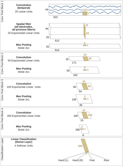
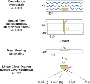
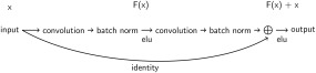
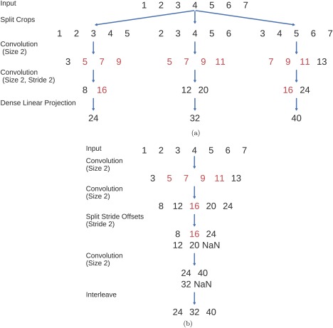
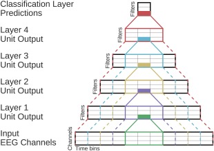
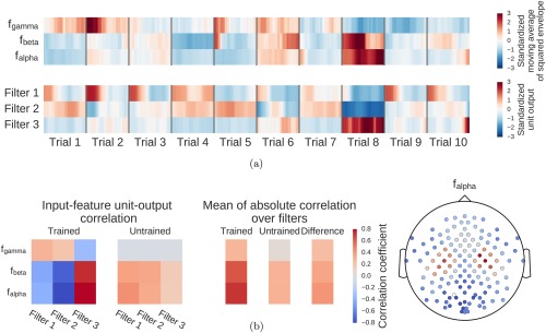
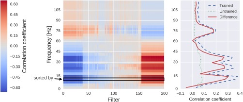
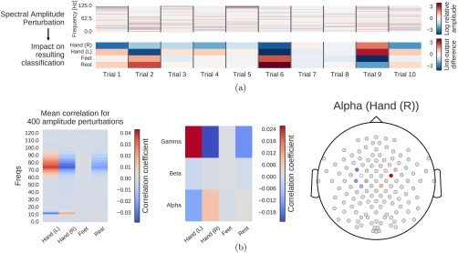
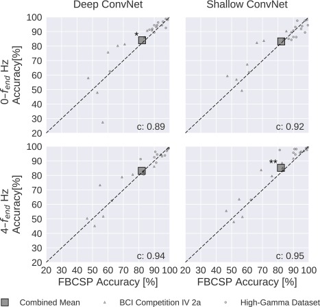
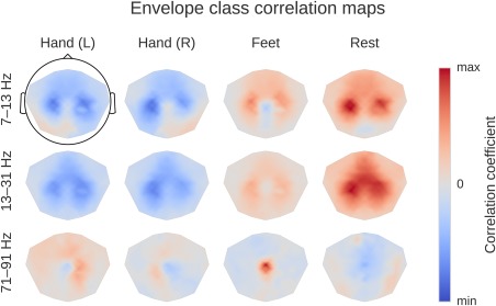
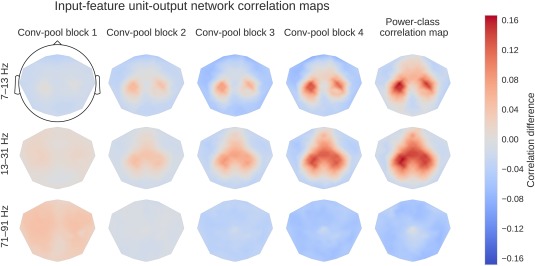
Deep learning with convolutional neural networks (deep ConvNets) has revolutionized computer vision through end-to-end learning, that is, learning from the raw data. There is increasing interest in using deep ConvNets for end-to-end EEG analysis, but a better understanding of how to design and train ConvNets for end-to-end EEG decoding and how to visualize the informative EEG features the ConvNets learn is still needed. Here, we studied deep ConvNets with a range of different architectures, designed for decoding imagined or executed tasks from raw EEG. Our results show that recent advances from the machine learning field, including batch normalization and exponential linear units, together with a cropped training strategy, boosted the deep ConvNets decoding performance, reaching at least as good performance as the widely used filter bank common spatial patterns (FBCSP) algorithm (mean decoding accuracies 82.1% FBCSP, 84.0% deep ConvNets). While FBCSP is designed to use spectral power modulations, the features used by ConvNets are not fixed a priori. Our novel methods for visualizing the learned features demonstrated that ConvNets indeed learned to use spectral power modulations in the alpha, beta, and high gamma frequencies, and proved useful for spatially mapping the learned features by revealing the topography of the causal contributions of features in different frequency bands to the decoding decision. Our study thus shows how to design and train ConvNets to decode task-related information from the raw EEG without handcrafted features and highlights the potential of deep ConvNets combined with advanced visualization techniques for EEG-based brain mapping. Hum Brain Mapp 38:5391-5420, 2017. © 2017 Wiley Periodicals, Inc.

Keywords: EEG analysis; brain mapping; brain-computer interface; brain-machine interface; electroencephalography; end-to-end learning; machine learning; model interpretability.

Figure 1

Deep ConvNet architecture. EEG input (at the top) is progressively transformed toward the bottom, until the final classifier output. Black cuboids: inputs/feature maps; brown cuboids: convolution/pooling kernels. The corresponding sizes are indicated in black and brown, respectively. Sizes are for the cropped training version, see the section “Architecture differences.” Each spatial filter has weights for all possible pairs of electrodes with filters of the preceding temporal convolution. Note that in these schematics, proportions of maps and kernels are only approximate. [Color figure can be viewed at http://wileyonlinelibrary.com]

Figure 2

Shallow ConvNet architecture. Conventions as in Figure 1. [Color figure can be viewed at http://wileyonlinelibrary.com]

Figure 3

Residual block. Residual block used in the ResNet architecture and as described in original paper (He et al. [2015]; see Fig. 2) with identity shortcut option A, except using ELU instead of ReLU nonlinearities. See the section “Residual ConvNet for raw EEG signals” for explanation.

Figure 4

Multiple‐crop prediction used for cropped training. In this toy example, a trial with the sample values 1,2,3,4,5,6,7 is cut into three crops of length 5 and these crops are passed through a convolutional network with two convolutional layers and one dense layer. The convolutional layers both have kernel size 2, and the second one additionally uses a stride of 2. Filters for both layers and the final dense layer have values 1,1. Red indicates intermediate outputs that were computed multiple times in the naïve implementation. Note that both implementations result in the same final outputs. (a) Naïve implementation by first splitting the trial into crops and passing the crops through the ConvNet independently. (b) Optimized implementation, computing the outputs for each crop in a single forward pass. Strides in the original ConvNet are handled by separating intermediate results that correspond to different stride offsets, see the split stride offsets step. NaNs are only needed to pad all intermediate outputs to the same size and are removed in the end. The split stride step can simply be repeated in case of further layers with stride. We interleave the outputs only after the final predictions, also in the case of ConvNets with more layers. [Color figure can be viewed at http://wileyonlinelibrary.com]

Figure 5

ConvNet Receptive Fields Schema. Showing the outputs, inputs, and receptive fields of one unit per layer. Colors indicate different units. Filled rectangles are individual units, and solid lines indicate their direct input from the layer before. Dashed lines indicate the corresponding receptive field in all previous layers including the original input layer. The receptive field of a unit contains all inputs that are used to compute the unit's output. The receptive fields get larger with increasing depth of the layer. Note that this is only a schema and exact dimensions are not meaningful in this figure. [Color figure can be viewed at http://wileyonlinelibrary.com]

Figure 6

Computation overview for input‐feature unit‐output network correlation map. (a) Feature inputs and unit outputs for input‐feature unit‐output correlation map. Moving average of squared envelopes and unit outputs for 10 trials. Upper rows show mean squared envelopes over the receptive field for three frequency ranges in the alpha, beta, and gamma frequency band, standardized per frequency range. Lower rows show corresponding unit outputs for three filters, standardized per filter. All time series standardized for the visualization. (b) Input‐feature unit‐output correlations and corresponding scalp map for the alpha band. Left: Correlation coefficients between unit outputs of three filters and mean squared envelope values over the corresponding receptive field of the units for three frequency ranges in the alpha (7–13 Hz), beta (13–31 Hz), and gamma (71–91 Hz) frequency band. Results are shown for the trained and the untrained ConvNet and for one electrode. Middle: Mean of the absolute correlation coefficients over the three filters for the trained and the untrained ConvNet, and the difference between trained and untrained ConvNet. Right: An exemplary scalp map for correlations in the alpha band (7–13 Hz), where the color of each dot encodes the correlation difference between a trained and an untrained ConvNet for one electrode. Note localized positive effects above areas corresponding to the right and left sensorimotor hand/arm areas, indicating that activity in these areas has large absolute correlations with the predictions of the trained ConvNet. [Color figure can be viewed at http://wileyonlinelibrary.com]

Figure 7

Correlation between the mean squared envelope feature and unit output for a single subject at one electrode position (FCC4h). Left: All correlations. Colors indicate the correlation between unit outputs per convolutional filter (x‐axis) and mean squared envelope in different frequency bands (y‐axis). Filters are sorted by their correlation to the 7–13 Hz envelope (outlined by the black rectangle). Note the large correlations/anticorrelations in the alpha/beta bands (7–31 Hz) and somewhat weaker correlations/anticorrelations in the gamma band (around 75 Hz). Right: mean absolute values across units of all convolutional filters for all correlation coefficients of the trained model, the untrained model and the difference between the trained and untrained model. Peaks in the alpha, beta, and gamma bands are clearly visible. [Color figure can be viewed at http://wileyonlinelibrary.com]

Figure 8

Computation overview for input‐perturbation network‐prediction correlation map. (a) Example spectral amplitude perturbation and resulting classification difference. Top: Spectral amplitude perturbation as used to perturb the trials. Bottom: unit‐output difference between unperturbed and perturbed trials for the classification layer units before the softmax. (b) Input‐perturbation network‐prediction correlations and corresponding network correlation scalp map for alpha band. Left: Correlation coefficients between spectral amplitude perturbations for all frequency bins and differences of the unit outputs for the four classes (differences between unperturbed and perturbed trials) for one electrode. Middle: Mean of the correlation coefficients over the the alpha (7–13 Hz), beta (13–31 Hz) and gamma (71–91 Hz) frequency ranges. Right: An exemplary scalp map for the alpha band, where the color of each dot encodes the correlation of amplitude changes at that electrode and the corresponding prediction changes of the ConvNet. Negative correlations on the left sensorimotor hand/arm areas show an amplitude decrease in these areas leads to a prediction increase for the Hand (R) class, whereas positive correlations on the right sensorimotor hand/arm areas show an amplitude decrease leads to a prediction decrease for the Hand (R) class. This complements the information from the input‐feature unit‐output network correlation map (Fig. 6b), which showed band power in these areas is strongly correlated with unit outputs in the penultimate layer. [Color figure can be viewed at http://wileyonlinelibrary.com]

Figure 9

FBCSP versus ConvNet decoding accuracies. Each small marker represents the accuracy of one subject, the large square markers represent average accuracies across all subjects of both datasets. Markers above the dashed line indicate experiments where ConvNets performed better than FBCSP and opposite for markers below the dashed line. Stars indicate statistically significant differences between FBCSP and ConvNets (Wilcoxon signed‐rank test, P < 0.05: *, P < 0.01: **, P < 0.001=***). Bottom left of every plot: linear correlation coefficient between FBCSP and ConvNet decoding accuracies. Mean accuracies were very similar for ConvNets and FBCSP, the (small) statistically significant differences were in direction of the ConvNets. [Color figure can be viewed at http://wileyonlinelibrary.com]

Figure 10

Confusion matrices for FBCSP‐ and ConvNet‐based decoding. Results are shown for the High‐Gamma Dataset, on 0–f_end Hz. Each entry of row r and column c for upper‐left 4×4‐square: Number of trials of target r predicted as class c (also written in percent of all trials). Bold diagonal corresponds to correctly predicted trials of the different classes. Percentages and colors indicate fraction of trials in this cell from all trials of the corresponding column (i.e., from all trials of the corresponding target class). The lower‐right value corresponds to overall accuracy. Bottom row corresponds to sensitivity defined as the number of trials correctly predicted for class c/number of trials for class c. Rightmost column corresponds to precision defined as the number of trials correctly predicted for class r/number of trials predicted as class r. Stars indicate statistically significantly different values of ConvNet decoding from FBCSP, diamonds indicate statistically significantly different values between the shallow and deep ConvNets. P<0.05: $\diamond$/*, P<0.01: $\diamond \diamond$/**, P<0.001: $\diamond \diamond \diamond$/***, Wilcoxon signed‐rank test. [Color figure can be viewed at http://wileyonlinelibrary.com]

Figure 11

Impact of ConvNet design choices on decoding accuracy. Accuracy differences of baseline and design choices on x‐axis for the 0–f_end‐Hz and 4–f_end‐Hz datasets. Each small marker represents accuracy difference for one subject, and each larger marker represents mean accuracy difference across all subjects of both datasets. Bars: standard error of the differences across subjects. Stars indicate statistically significant differences to baseline (Wilcoxon signed‐rank test, P < 0.05: *, P < 0.01: **, P < 0.001=***). (a) Impact of design choices applicable to both ConvNets. Shown are the effects from the removal of one aspect from the architecture on decoding accuracies. All statistically significant differences were accuracy decreases. Notably, there was a clear negative effect of removing both dropout and batch normalization, seen in both ConvNets' accuracies and for both frequency ranges. (b) Impact of different types of nonlinearities, pooling modes and filter sizes. Results are given independently for the deep ConvNet and the shallow ConvNet. As before, all statistically significant differences were from accuracy decreases. Notably, replacing ELU by ReLU as nonlinearity led to decreases on both frequency ranges, which were both statistically significant. [Color figure can be viewed at http://wileyonlinelibrary.com]

Figure 12

Impact of recent advances on overall decoding accuracies. Accuracies without batch normalization, dropout and ELUs. All conventions as in Figure 9. In contrast to the results on Figure 9, the deep ConvNet without implementation of these recent methodological advances performed worse than FBCSP; the difference was statistically significant for both frequency ranges. [Color figure can be viewed at http://wileyonlinelibrary.com]

Figure 13

Impact of training strategy (cropped vs trial‐wise training) on accuracy. Accuracy difference for both frequency ranges and both ConvNets when using cropped training instead of trial‐wise training. Other conventions as in Figure 11. Cropped training led to better accuracies for almost all subjects for the deep ConvNet on the 4–f_end‐Hz frequency range. [Color figure can be viewed at http://wileyonlinelibrary.com]

Figure 14

Envelope‐class correlations for alpha, beta, and gamma bands for all classes. Average over subjects from the High‐Gamma Dataset. Colormaps are scaled per frequency band/row. This is a ConvNet‐independent visualization, for an explanation of the computation see the section “Input‐feature unit‐output correlation maps.” Scalp plots show spatial distributions of class‐related spectral amplitude changes well in line with the literature. [Color figure can be viewed at http://wileyonlinelibrary.com]

Figure 15

Power input‐feature unit‐output network correlation maps for all conv‐pool blocks of the deep ConvNet. Correlation difference indicates the difference of correlation coefficients obtained with the trained and untrained model for each electrode respectively and is visualized as a topographic scalp plot. For details, see the section “Input‐feature unit‐output correlation maps.” Rightmost column shows the correlation between the envelope of the EEG signals in each of the three analyzed frequency bands and the four classes. All colormaps are on the same scale. Notably, the absolute values of the correlation differences became larger in the deeper layers and converged to patterns that were very similar to those obtained from the power–class correlations. [Color figure can be viewed at http://wileyonlinelibrary.com]

Figure 16

Absolute correlations between unit outputs and class labels. Each dot represents absolute correlation coefficients for one layer of the deep ConvNet. Solid lines indicate result of taking mean over absolute correlation coefficients between classes and filters. Dashed lines indicate result of first taking the maximum absolute correlation coefficient per class (maximum over filters) and then the mean over classes. Absolute correlations increased almost linearly with increasing depth of the layer. [Color figure can be viewed at http://wileyonlinelibrary.com]

Figure 17

Input‐perturbation network‐prediction correlations for all frequencies for the deep ConvNet, per class. Plausible correlations, for example, rest positively, other classes negatively correlated with the amplitude changes in frequency range from 20 to 30 Hz. [Color figure can be viewed at http://wileyonlinelibrary.com]

Figure 18

Absolute input‐perturbation network‐prediction correlation frequency profile for the deep ConvNet. Mean absolute correlation value across classes. CSP binary decoding accuracies for different frequency bands for comparison, averaged across subjects and class pairs. Peaks in alpha, beta, and gamma band for input‐perturbation network‐prediction correlations and CSP accuracies. [Color figure can be viewed at http://wileyonlinelibrary.com]

Figure 19

Input‐perturbation network‐prediction correlation maps for the deep ConvNet. Correlation of class predictions and amplitude changes. Averaged over all subjects of the High‐Gamma Dataset. Colormaps are scaled per scalp plot. Plausible scalp maps for all frequency bands, for example, contralateral positive correlations for the hand classes in the gamma band. [Color figure can be viewed at http://wileyonlinelibrary.com]

References

1. Abdel‐Hamid O, Mohamed A. r, Jiang H, Deng L, Penn G, Yu D (2014): Convolutional neural networks for speech recognition. IEEE/ACM Trans Audio Speech Lang Process 22:1533–1545.
1. Ang KK, Chin ZY, Zhang H, Guan C (2008): Filter Bank Common Spatial Pattern (FBCSP) in Brain‐Computer Interface. In IEEE International Joint Conference on Neural Networks, 2008. IJCNN 2008. (IEEE World Congress on Computational Intelligence), pp 2390–2397.
1. Antoniades A, Spyrou L, Took CC, Sanei S (2016): Deep learning for epileptic intracranial EEG data. In 2016 IEEE 26th International Workshop on Machine Learning for Signal Processing (MLSP), pp 1–6.
1. Bach S, Binder A, Montavon G, Klauschen F, Müller K‐R, Samek W (2015): On pixel‐wise explanations for non‐linear classifier decisions by layer‐wise relevance propagation. PLoS ONE 10:e0130140. - PMC - PubMed
1. Ball T, Demandt E, Mutschler I, Neitzel E, Mehring C, Vogt K, Aertsen A, Schulze‐Bonhage A (2008): Movement related activity in the high gamma range of the human EEG. NeuroImage 41:302–310. - PubMed
Publication types