Structure in neural population recordings: an expected byproduct of simpler phenomena?

Abstract

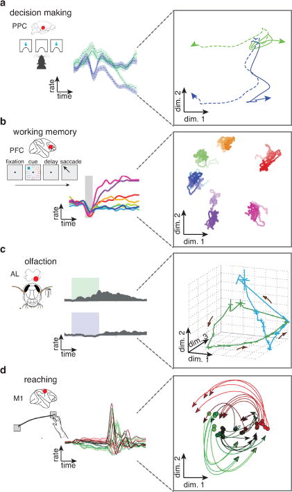
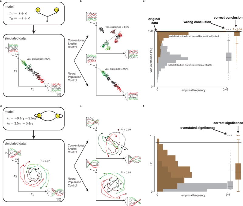
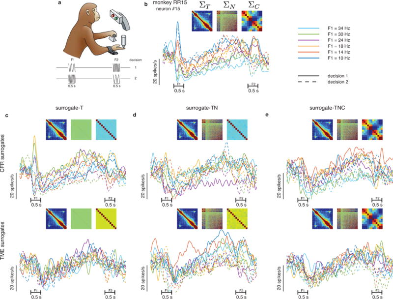
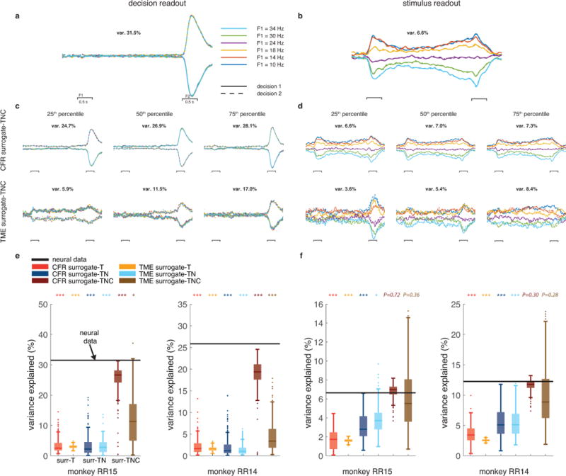
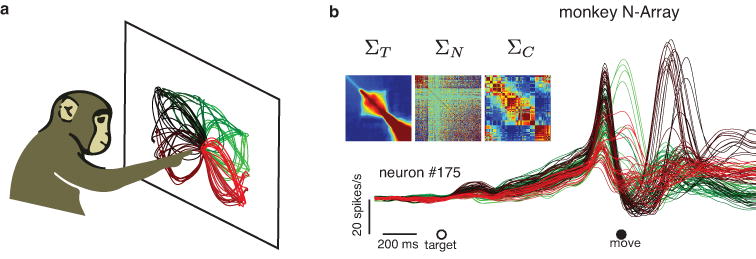
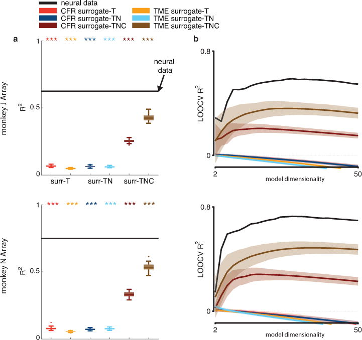
Neuroscientists increasingly analyze the joint activity of multineuron recordings to identify population-level structures believed to be significant and scientifically novel. Claims of significant population structure support hypotheses in many brain areas. However, these claims require first investigating the possibility that the population structure in question is an expected byproduct of simpler features known to exist in data. Classically, this critical examination can be either intuited or addressed with conventional controls. However, these approaches fail when considering population data, raising concerns about the scientific merit of population-level studies. Here we develop a framework to test the novelty of population-level findings against simpler features such as correlations across times, neurons and conditions. We apply this framework to test two recent population findings in prefrontal and motor cortices, providing essential context to those studies. More broadly, the methodologies we introduce provide a general neural population control for many population-level hypotheses.

Figure 1. Population structure in systems neuroscience

Examples from studies investigating structure at the level of the population. (a) Left panel shows an example firing rate response from a rat posterior parietal cortex neuron during a multi-modality decision-making task, adapted from Raposo et al.. The single-neuron responses show mixed selectivity to cue modality (blue: visual cue; green: auditory cue) and decision (dashed lines, right lick port; solid lines, left lick port). Right panel shows a two-dimensional projection of the population response, where choice information is separated along dimension 1 (horizontal) from the modality information, which is separated along dimension 2 (vertical). (b) Left panel shows an example firing rate response from a primate prefrontal cortex neuron during a working memory task, adapted from Murray et al.. The single-neuron responses at the six stimuli (illustrated by different colors) show temporal dynamics. Right panel shows a two-dimensional projection of the population where stimulus information is stably represented across time. (c) Left panel shows an example firing rate response from a locust antennal lobe projection neuron responding to two odors, adapted from Broome et al.. Right panel shows a three-dimensional projection of the population data with neural trajectories corresponding to the two odor stimuli. (d) Left panel shows an example firing rate response from a primate motor cortex neuron during a delayed-reach task, adapted from Churchland et al.. Right panel shows a two-dimensional projection of the population data with neural trajectories corresponding to each reaching condition.

Figure 2. Motivation for the neural population control

(a) Simulated firing rates from two neurons encoding a hypothetical stimulus at eight conditions (high, moderate, and low stimuli correspond to red, black, and green color shades, respectively) are shown, along with the corresponding neural trajectories in the population space (here two-dimensional). Black line illustrates a one-dimensional projection of the data that represents stimulus, identified by the target dimensionality reduction method from Mante et al.. The data variance explained by this projection is shown (as a percentage). (b) Top panel shows shuffled surrogate data generated by shuffling the single neuron responses from panel a across conditions. The same data analysis method was then used to identify a one-dimensional projection of the data (black line) that represents the stimulus in the shuffled data. Bottom panel shows random surrogate data from the neural population control (Methods, to be described), and the identified projection that represents the stimulus (black line). (c) Distribution of variance-explained values from stimulus projections identified from 1000 surrogate datasets (gray) and another distribution of variance values from 1000 surrogate datasets from the neural population control (brown). Black line is the percentage variance explained from the neural data from panel a. Box-whisker plots summarize the two distributions (Tukey convention). (d) Firing rates for two neurons are solutions to the given differential equations (modeling an oscillator), with eight different initial conditions. The fit of these data to a linear system (R²) is shown. (e) Shuffled data (top) and surrogate data from the neural population control. (f) Distributions of R² values from 1000 shuffled datasets and 1000 surrogate datasets from the neural population control (same convention as panel c). Smoothed Gaussian noise was added to all simulated data.

Figure 3. CFR and TME surrogate datasets preserve the specified primary features

(a) Working memory task, adapted from Romo and Salinas. (b) Example neuron (neuron number 15 of 571 total) from prefrontal cortex. Each trace is the trial-averaged firing of the twelve task conditions (six stimuli and two decisions; one trace color and style for each). Horizontal bars denote the times of first (F1) and second (F2) vibrotactile stimuli. Heatmaps in the inset show three covariance matrices across times ( ${\sum }_T$), neurons ( ${\sum }_N)$and conditions $\left({\sum }_C\right)$ of all neurons in this dataset. (c-e) Example neurons from one surrogate-T, surrogate-TN, and surrogate-TNC dataset, respectively; with the same conventions as panel b. Top panels in c-e are surrogate datasets generated using the Corrected Fisher Randomization method (CFR) and bottom panels in c-e are surrogate datasets generated using the Tensor Maximum Entropy method (TME). The covariance matrices in the insets in c-e are obtained by averaging the primary features from 100 surrogate datasets.

Figure 4. Decision (stimulus) readouts in PFC are not (are) an expected byproduct

The population readouts for decision and stimulus were identified using demixed principle component analysis (dPCA). (a) Projections of the original population responses from monkey RR15 onto the top decision-specific readout. (b) Projections of neural responses from monkey RR15 onto the top stimulus-specific readout. The trace colors and style follows the same convention as those in Fig. 3b. (c) Same as a but for decision readouts from surrogate datasets generated by CFE (top) and TME (bottom). We show surrogates at various points in the distribution of variance explained (25^th, 50^th, and 75^th percentile, 200 surrogate datasets). (d) Same as b but for the surrogate datasets from CFE (top) and TME (bottom) methods; as in c the 25^th, 50^th, and 75^th percentile examples are shown (200 surrogate datasets). Scale bars and color scheme in b-d match the scale bars and color scheme in a. (e) Percent variance-explained of the population projection onto the top decision readout. Black lines show the percent variance explained from the original neural data, colored box-whisker plots show the variance explained distribution from 200 surrogate samples (same convention as Fig. 2 c,f; stars denote significantly high variance; upper-tail test). The variance of the decision projection is calculated during the decision epoch (100 ms after the second stimulus onset, until the second stimulus offset). (f) Same as e but for percent variance explained of the population projection onto the top stimulus readout. The variance of the stimulus projection is calculated during the stimulus epoch (100 ms after first stimulus onset, until the second stimulus onset).

Figure 5. Motor cortex responses during a delayed-reach task

(a) Delayed-reach task. Monkeys performed straight and curved reaches to targets displayed on a frontoparallel screen. Trajectories represent the average hand position during each of 108 reaching conditions. (b) Example neuron (neuron number 175 of 218 total) recorded from the motor cortex of one monkey during the delayed-reach task. Each trace is the smoothed, trial-averaged firing rate during one of the reaching conditions. The trace color indicates the reach condition from panel a. Heatmaps in the inset represent three covariance matrices that quantify the primary features across time ( ${\sum }_T$), neurons ( ${\sum }_N)$and conditions $\left({\sum }_C\right)$ of the entire population dataset.

Figure 6. Population dynamics in motor cortex are not an expected byproduct

400 ms of movement-related neural activity in the motor cortex were projected on to the top principal components (PCs) and then fitted to a linear dynamical system. (a) Quality of fit (R²) of the original neural responses projected onto the top 28 PCs (determined by cross validation; Supplementary Fig. 8) to the dynamical system model. Black lines denote the R² from the original neural data. Colored box-whisker plots denote the R² distributions from 100 surrogate datasets from each surrogate type (same convention as Fig. 2 c,f). Stars denote significantly higher R² than the surrogates (P<0.001; upper-tail test). (b) Leave-one-condition-out cross-validation (LOOCV) for the R² measure of fitting data to a dynamical system model with different choices of model dimensionalities (number of PCs). Black trace denote the R² value from the original neural data and colored traces are the mean R² values from the surrogate datasets (same color convention as panel a. (Colored areas represent $\pm 2\mathrm{s}.\mathrm{d}.$

References

1. Cunningham JP, Yu BM. Dimensionality reduction for large-scale neural recordings. Nature Neuroscience. 2014;17:1500–1509. - PMC - PubMed
1. Gao PR, Ganguli S. On simplicity and complexity in the brave new world of large-scale neuroscience. Curr Opin Neurobiol. 2015;32:148–155. - PubMed
1. Stevenson IH, Kording KP. How advances in neural recording affect data analysis. Nature Neuroscience. 2011;14:139–142. - PMC - PubMed
1. Pillow JW, Shlens J, Paninski L, et al. Spatio-temporal correlations and visual signalling in a complete neuronal population. Nature. 2008;454:995–999. - PMC - PubMed
1. Stopfer M, Jayaraman V, Laurent G. Intensity versus identity coding in an olfactory system. Neuron. 2003;39:991–1004. - PubMed
LinkOut - more resources