Repliscan: a tool for classifying replication timing regions

Abstract

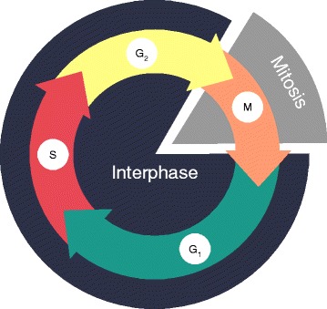
Background: Replication timing experiments that use label incorporation and high throughput sequencing produce peaked data similar to ChIP-Seq experiments. However, the differences in experimental design, coverage density, and possible results make traditional ChIP-Seq analysis methods inappropriate for use with replication timing.

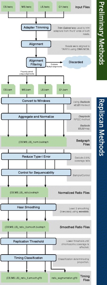
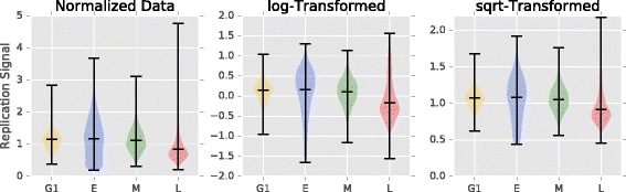
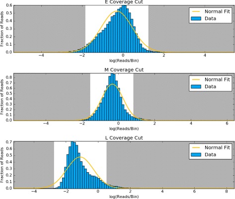
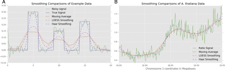
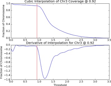
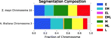
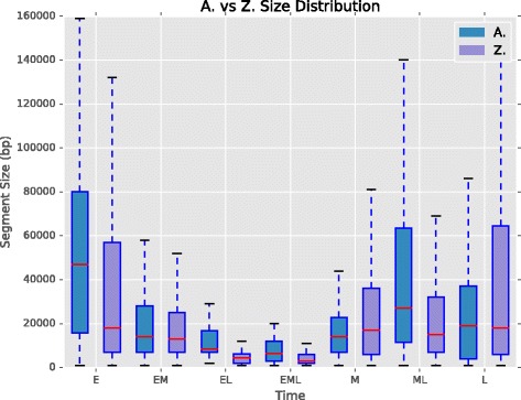
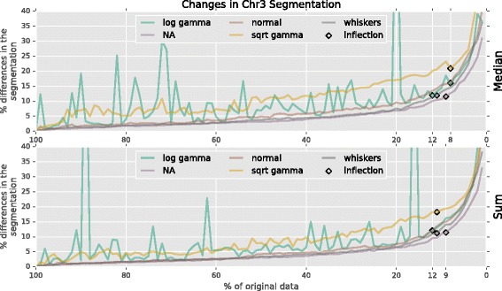
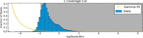
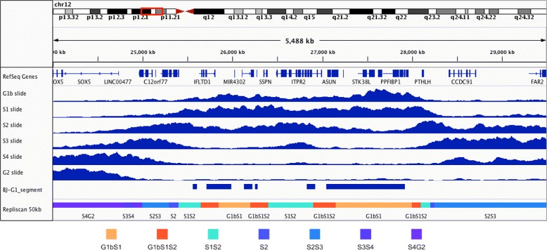
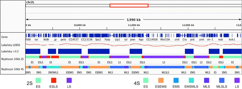
Results: To accurately detect and classify regions of replication across the genome, we present Repliscan. Repliscan robustly normalizes, automatically removes outlying and uninformative data points, and classifies Repli-seq signals into discrete combinations of replication signatures. The quality control steps and self-fitting methods make Repliscan generally applicable and more robust than previous methods that classify regions based on thresholds.

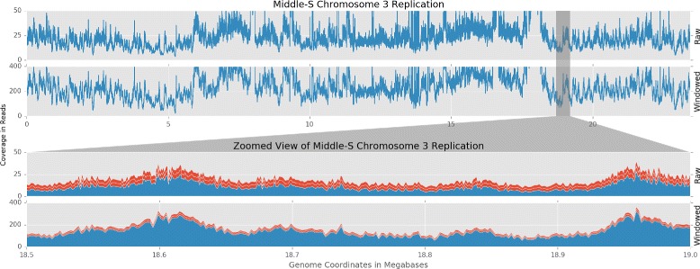
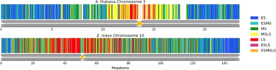
Conclusions: Repliscan is simple and effective to use on organisms with different genome sizes. Even with analysis window sizes as small as 1 kilobase, reliable profiles can be generated with as little as 2.4x coverage.

Keywords: Classification; DNA replication; Repli-seq.

Fig. 1

Overview of the cell cycle. Cell division takes place in two stages: interphase and mitosis. Interphase is when a cell copies its genome in preparation to physically divide during mitosis. Interphase starts with cell growth and preparation for DNA synthesis in Gap (G1). After G1, DNA is replicated in regions during the Synthesis (S) phase. The cell then transitions into a second growth phase - Gap 2 (G2). When the cell has finished growing, the cell divides into two daughter cells in Mitosis (M)

Fig. 2

Repliscan workflow. Diagram of the preliminary alignment and quality control methods at the top, and the Repliscan methods at the bottom

Fig. 3

Replication signal and sampling uncertainty. The top two graphs show raw and windowed replication signal across A. thaliana chromosome 3. The bottom two graphs show raw and windowed replications signals at 18.5-19.0 megabases from the top view as represented by the gray selection area. The red bars represent sampling uncertainty ($\sqrt{\lambda }$ for Poisson distributions)

Fig. 4

Normalized and transformed replication signals. Violin plots showing how the normalized and aggregated A. thaliana chromosome 3 replication signals from G1, early (E), middle (M), and late (L) S-phase data was bounded from [0,∞). We separately experimented with with log transforms to make the distributions more normal-like, and square root transforms to stabilize the spread

Fig. 5

Outlying coverage in chromosome 3. Based on the normal distribution fit (yellow) to the log transformed coverage distribution of early (E), middle (M), and late (L) S-phase data, windows that fall in the tails shaded in gray are removed from the analysis

Fig. 6

Smoothing comparisons. a - Noise (green) is added to an original signal (purple), and then smoothed with a 4 unit (40 point) moving average (orange), a 5 unit (25% subset) LOESS (red), and a level 3 Haar wavelet (blue). Both the moving average and LOESS spread out the peaks and artificially lowered signal amplitudes, while the Haar wavelet keeps bounds and peak heights close to the original. b - The A. thaliana middle S-phase normalized signal (green), is smoothed with a moving average (orange), LOESS (red), and the level 3 Haar wavelet (blue) for comparison

Fig. 7

Replication threshold from coverage. The upper plot shows how much of A. thaliana chromosome 3 will be kept for downstream analysis as a function of the signal threshold. The lower plot shows the chromosome coverage differential as a function of the threshold. The vertical red line in each plot marks the optimal threshold of 0.92

Fig. 8

Comparison of A. thaliana and Z. mays segmentation. Following the segmentation legend on the right, A. thaliana chromosome 3 (top) and Z. mays chromosome 10 (bottom) have been classified into segmentation regions by Repliscan. The large white regions in the A. thaliana figure are unclassified regions due to high or very low signal. Below each replication segmentation is a depiction of the chromosome, with the centromere location marked in yellow [32, 33]

Fig. 9

Composition of replication segmentation. The segment composition shows that replication in A. thaliana is skewed towards early S replication, while Z. mays has an even distribution across early, middle, and late S. We can also see that the non-sequential early-late (EL) and early-middle-late (EML) classifications comprise a very small proportion of the classified segments in both cases

Fig. 10

Segment size distribution. Boxplots for every combination of replication time, illustrating the distribution of segment sizes. Early (E) and mid-late (ML) S were largest in A. thaliana, while early and late (L) were largest in Z. mays

Fig. 11

Segmentation differences in downsampled data. After downsampling the A. thaliana data, the accuracy of median (top) and sum (bottom) aggregation, and outlier detection using log gamma, none (NA), normal, square root gamma, and whiskers. Inflection points in the differences are labeled with black diamonds

Fig. 12

Unconverged log gamma fit. Most of the data is removed when the iterative fitting function fails to converge with the log transformed gamma distribution. Instances like this produce the spikes of differences in Fig. 11

Fig. 13

Human fibroblast Repli-seq. 50 kilobase sliding window replication signals (blue) reproduced from Hansen et al., published “BJ-G1_segment” regions, and 50 kilobase Repliscan results (bottom)

Fig. 14

D. melanogaster KC167 Repli-Seq. Reproduction of the LOESS smoothed continuous replication profile (Lubelsky LOESS), and the thresholded, discrete early (blue) and late timing domains (Lubelsky > 0.5) from original Lubelsky et al. study. Repliscan segmentation results with Early (Early, Early-Mid) and Late (Mid-Late, Late) replication (2S), and Early, Early-Mid, Mid-Late, and Late replication (4S) configuration with 10 kilobase windows

References

1. Alberts B, Johnson A, Lewis J, Raff M, Roberts K, Walter P. Molecular Biology of the Cell. New York: Garland Science; 2002.
1. Hand R. Eucaryotic dna: organization of the genome for replication. Cell. 1978;15(2):317–25. doi: 10.1016/0092-8674(78)90001-6. - DOI - PubMed
1. Rhind N, Gilbert DM. Dna replication timing. Cold Spring Harb Perspect Biol. 2013;5(8):010132. doi: 10.1101/cshperspect.a010132. - DOI - PMC - PubMed
1. Hansen RS, Canfield TK, Lamb MM, Gartler SM, Laird CD. Association of fragile x syndrome with delayed replication of the fmr1 gene. Cell. 1993;73(7):1403–9. doi: 10.1016/0092-8674(93)90365-W. - DOI - PubMed
1. Woodfine K, Fiegler H, Beare DM, Collins JE, McCann OT, Young BD, Debernardi S, Mott R, Dunham I, Carter NP. Replication timing of the human genome. Hum Mol Genet. 2004;13(2):191–202. doi: 10.1093/hmg/ddh016. - DOI - PubMed