On transient climate change at the Cretaceous-Paleogene boundary due to atmospheric soot injections

Abstract

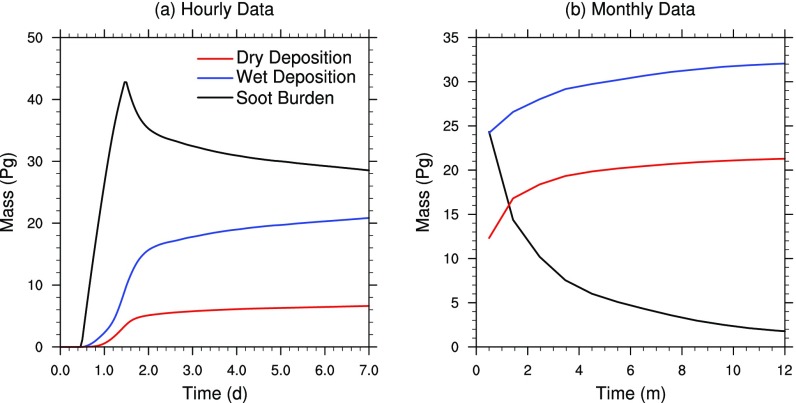
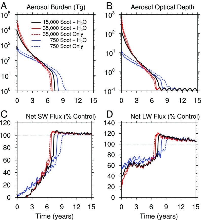
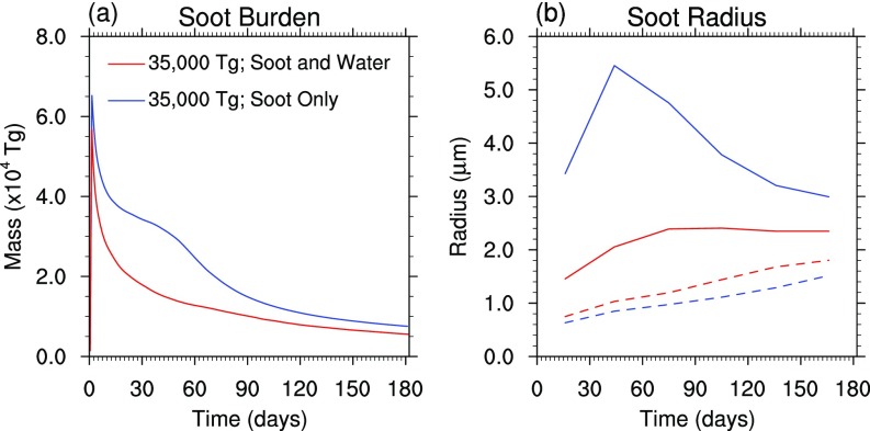
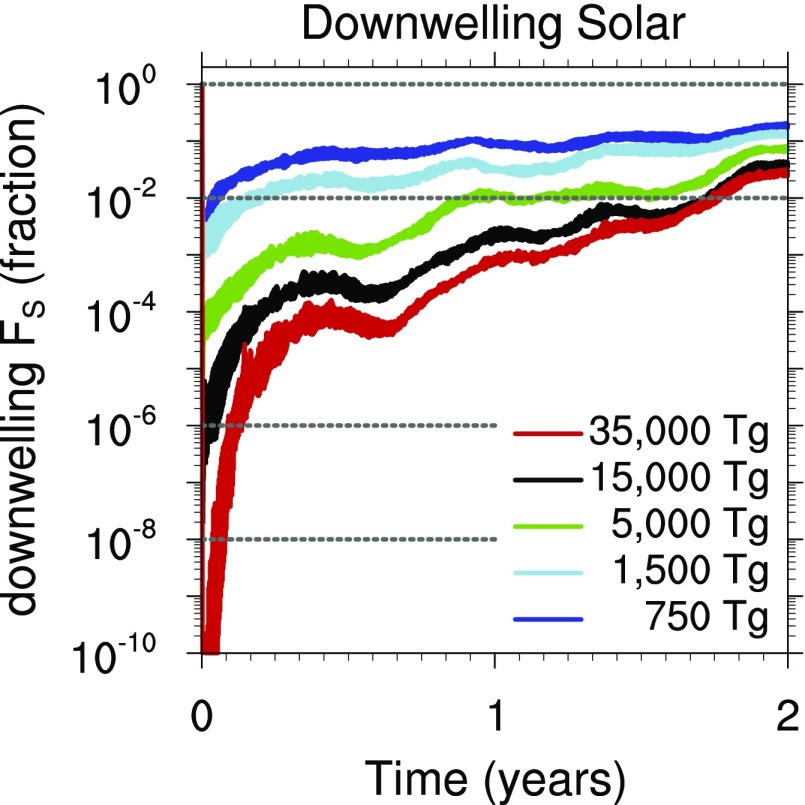
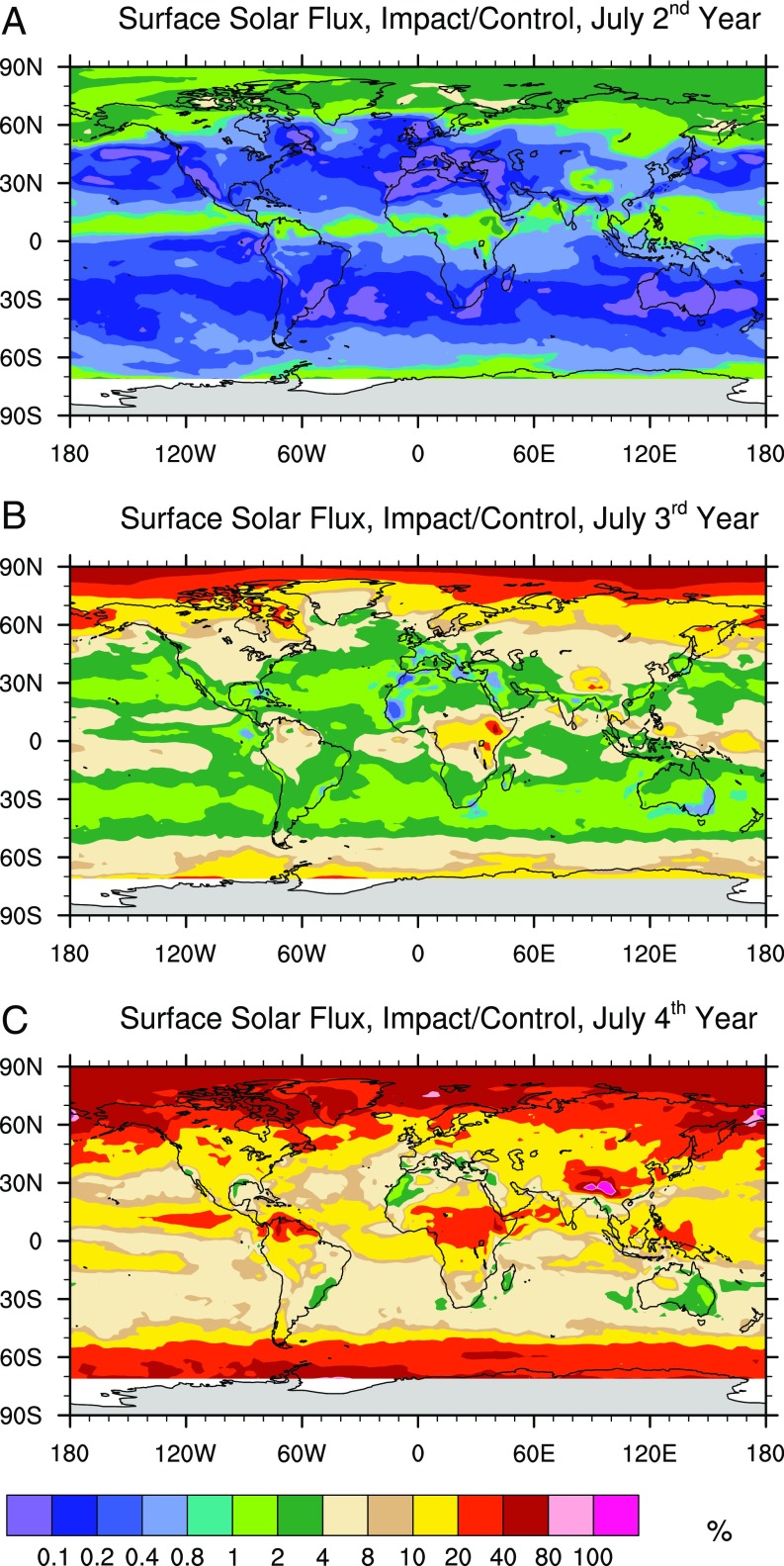
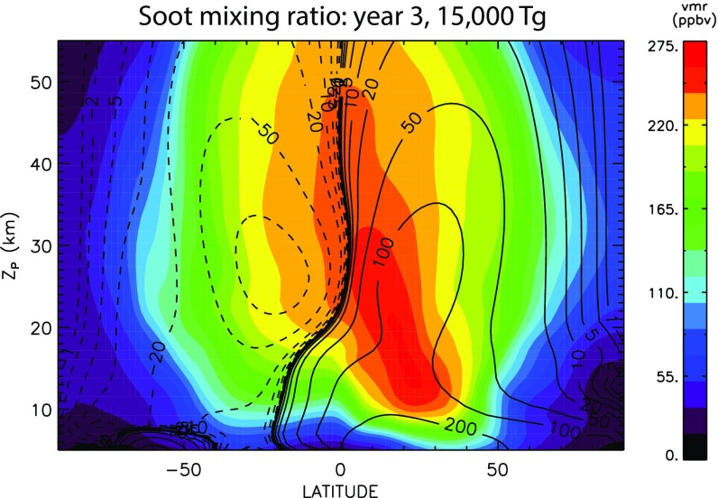
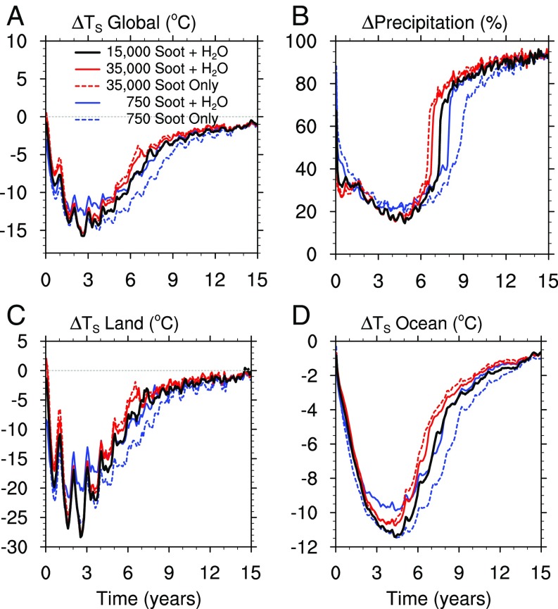
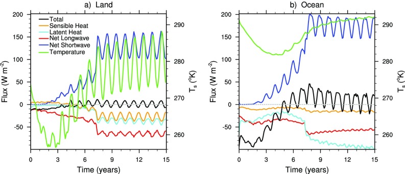
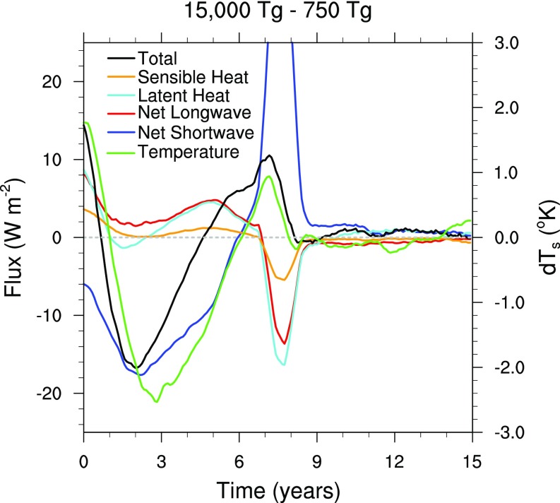
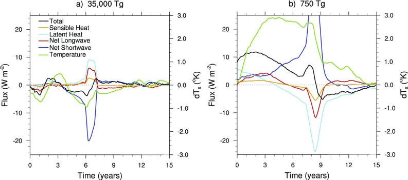
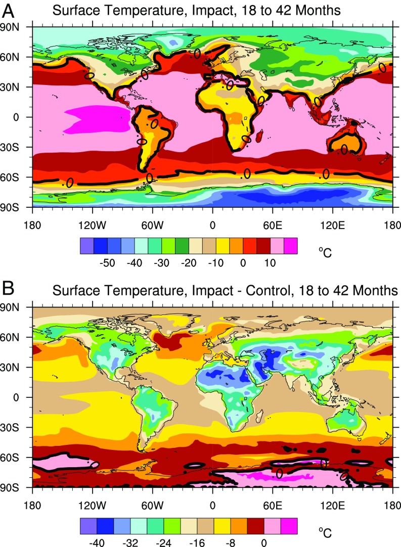
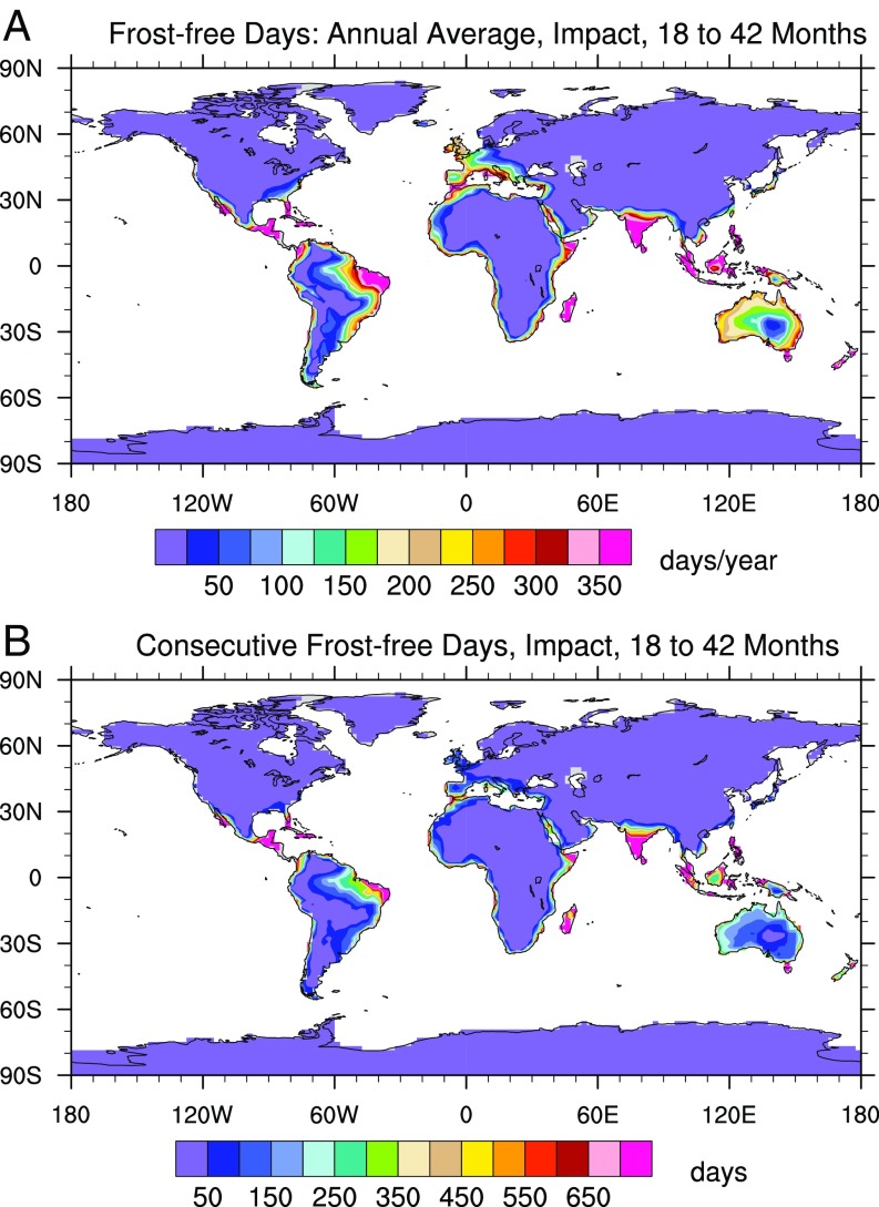
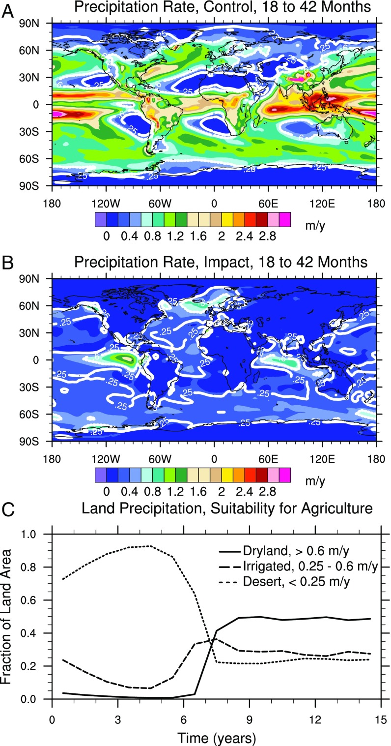
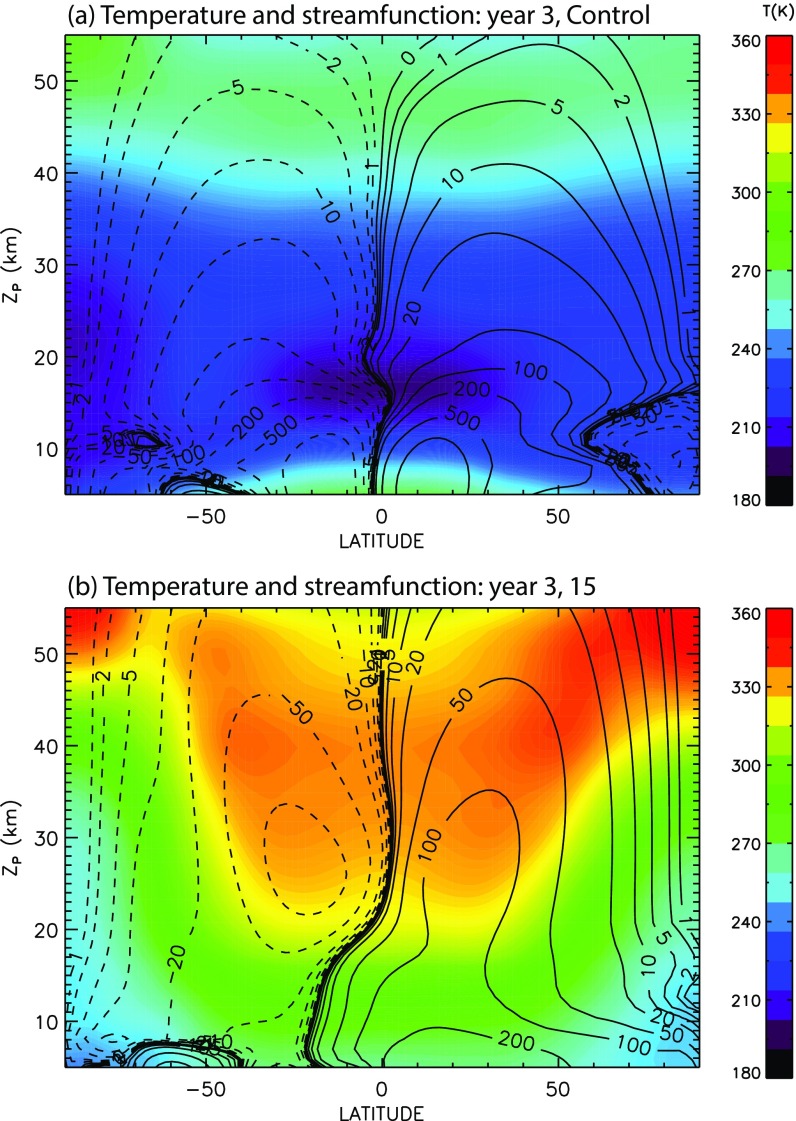
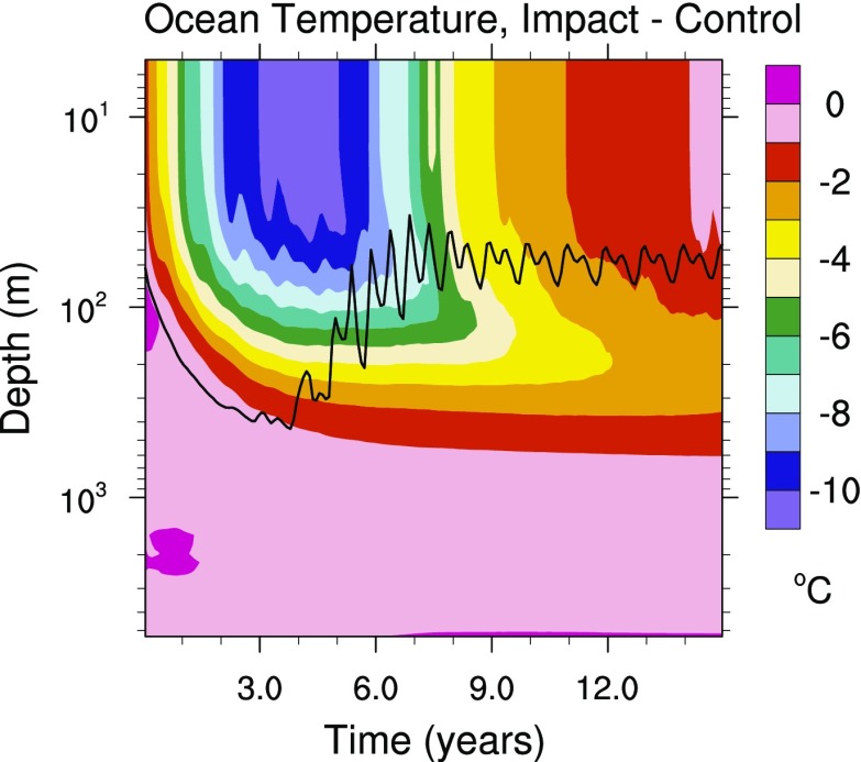
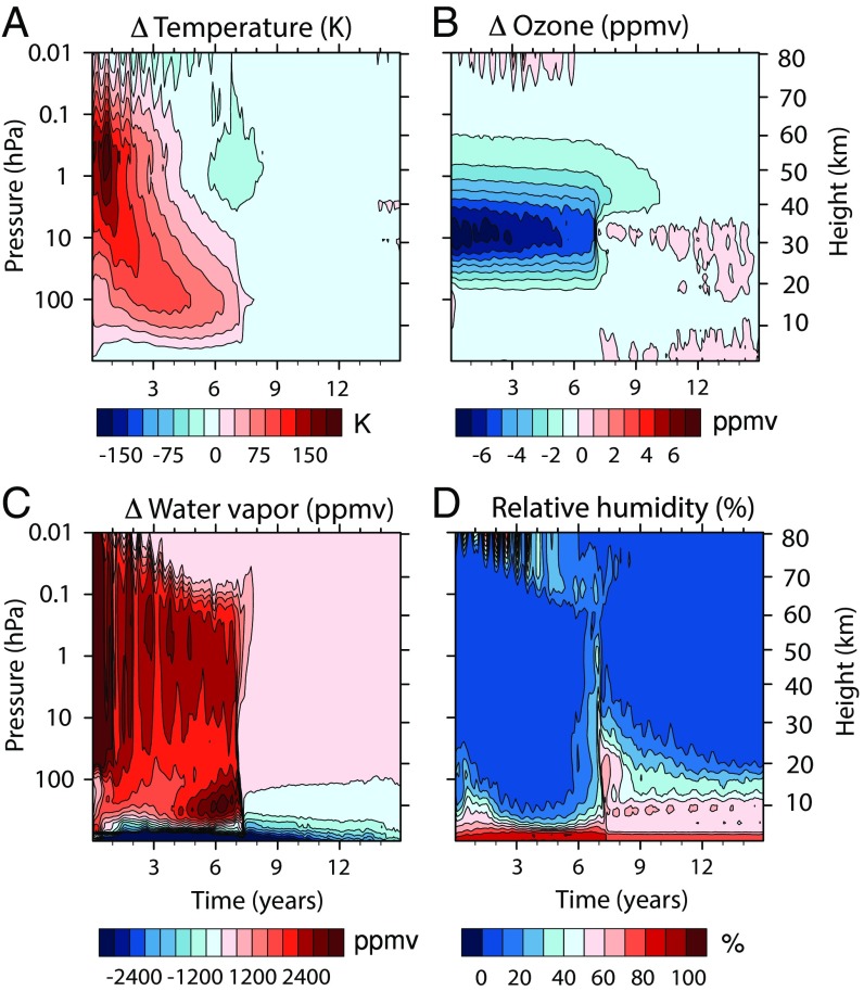
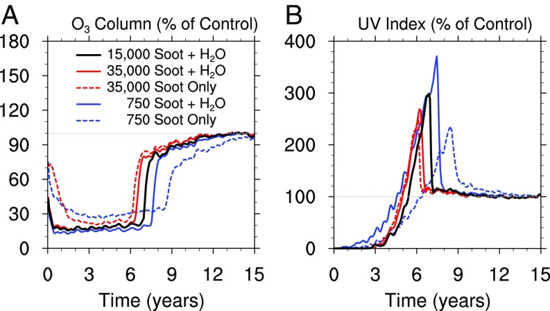
Climate simulations that consider injection into the atmosphere of 15,000 Tg of soot, the amount estimated to be present at the Cretaceous-Paleogene boundary, produce what might have been one of the largest episodes of transient climate change in Earth history. The observed soot is believed to originate from global wildfires ignited after the impact of a 10-km-diameter asteroid on the Yucatán Peninsula 66 million y ago. Following injection into the atmosphere, the soot is heated by sunlight and lofted to great heights, resulting in a worldwide soot aerosol layer that lasts several years. As a result, little or no sunlight reaches the surface for over a year, such that photosynthesis is impossible and continents and oceans cool by as much as 28 °C and 11 °C, respectively. The absorption of light by the soot heats the upper atmosphere by hundreds of degrees. These high temperatures, together with a massive injection of water, which is a source of odd-hydrogen radicals, destroy the stratospheric ozone layer, such that Earth's surface receives high doses of UV radiation for about a year once the soot clears, five years after the impact. Temperatures remain above freezing in the oceans, coastal areas, and parts of the Tropics, but photosynthesis is severely inhibited for the first 1 y to 2 y, and freezing temperatures persist at middle latitudes for 3 y to 4 y. Refugia from these effects would have been very limited. The transient climate perturbation ends abruptly as the stratosphere cools and becomes supersaturated, causing rapid dehydration that removes all remaining soot via wet deposition.

Keywords: Chicxulub; Cretaceous; asteroid impact; extinction; soot.

Fig. S1.

Evolution of soot burden (black) and cumulative wet (blue) and dry (red) deposition for the simulation with 15,000 Tg of fine soot and 41,000 Tg of coarse soot, including injections of H₂O, CO₂, and heat from fires for (A) 1 wk using hourly data and (B) 1 y using monthly average data. The soot is emitted over the first 12 h to 36 h and is followed by rapid wet and dry removal. After 1 y, the remaining soot burden is 4% of the total 56,000-Tg emission, with 57% removed by wet deposition and 38% removed by dry deposition.

Fig. 1.

Simulated changes in several important climate parameters following injections of 750 Tg and 35,000 Tg of soot near the tropopause, as well as cases that include water vapor injections for 750 Tg, 15,000 Tg, and 35,000 Tg. (A) Aerosol burden, (B) Aerosol optical depth, (C) net shortwave (SW) flux, and (D) net longwave (LW) flux. All parameters are monthly and globally averaged. Optical depth is calculated at 500 nm, near the center of the visible range of wavelength. Net SW and LW fluxes are shown as fractions of the value in the control simulation at Earth’s surface.

Fig. S2.

(A) Soot burden and (B) effective soot particle radius for the first 6 mo of the two 35,000-Tg simulations (with and without the addition of water vapor). Soot burden is from instantaneous, hourly model output; soot radius is from monthly average output. The soot radius shown is the equivalent spherical radius at 100 hPa (solid) and 10 hPa (dashed). When water accompanies the soot injection, a very large amount of soot is removed by precipitation within a few days (A, red curve). In the simulation without water vapor, rapid removal of soot starts around day 60, due to coagulation and sedimentation of large particles (A, blue curve). This effect is seen at 100 hPa but does not occur at 10 hPa, where the mixing ratio of soot is much smaller and very large particles do not form (B).

Fig. 2.

Ratio of downwelling solar flux at the surface from soot injections of 750 Tg, 1,500 Tg, 5,000 Tg, 15,000 Tg, and 35,000 Tg to its value in the control run. All time series use instantaneous hourly data. All cases include injection of water vapor.

Fig. 3.

Solar flux at the surface for the 15,000-Tg soot plus water simulation in July of the (A) second, (B) third, and (C) fourth years following the impact. The flux is shown as a percentage of the control case.

Fig. S3.

Aerosol loading (volume mixing ratio, parts per million by volume) and transformed Eulerian mean (TEM) meridional stream function (in kilograms per meter per second) in the stratosphere averaged over the third year after the impact. Positive stream function contours denote clockwise motion, and negative contours denote counterclockwise motion. Note the smaller aerosol loading at high latitudes.

Fig. 4.

As in Fig. 1, but for differences in global average (A) surface temperature, (C) land temperature, and (D) ocean temperature; and (B) global average precipitation as a fraction of the control simulation.

Fig. S4.

Evolution of average net surface energy fluxes and surface temperature (green; right ordinate scale) for the 15,000-Tg case over (A) the land and (B) the ocean. The total (black) is the sum of all of the flux terms, and is indicative of the net flux imbalance of the atmosphere−surface system; its sign is a measure of the energy loss or gain of the land and ocean. Surface temperature decreases rapidly following the reduction of shortwave flux, and reaches a minimum in year 3 over the land and years 4 to 5 over the ocean. Because of its much higher heat capacity, the ocean responds to the net energy loss by a smaller change in the global mean ocean temperature, which is reflected in the smaller change in ocean surface temperature compared with the land. Sensible and latent heat fluxes and net longwave radiation (orange, cyan, and red curves, respectively) from the colder surface decrease and mitigate the impact of the reduced solar flux. Over the land, the net surface flux remains close to equilibrium, as the very cold surface temperatures shut down heat loss via longwave, sensible, and latent heat fluxes. The sensible heat flux actually becomes slightly positive over the land, indicating that advection of relatively warmer air from the ocean warms the free atmosphere sufficiently to warm the land surface via sensible heat flux. Over the land, surface energy is being lost after the impact mostly as longwave radiation (red curves), while, over the ocean, longwave radiation and latent heat (cyan curves) contribute comparably to energy loss. Nonetheless, the reduction in latent heat flux is particularly large over the ocean because surface saturation has increased due to the combination of surface cooling and water vapor injected into the troposphere. During the third year after the 15,000-Tg soot injection, there is a gradual increase in net shortwave flux as the soot settles out of the atmosphere, returning to normal levels in year 7, when the remaining soot is rapidly removed. After 12 y to 15 y, the net surface flux in the 15,000-Tg case, as well as its seasonal cycle, approaches the values seen in the control case, although the surface temperature of the ocean is still a little colder than normal.

Fig. S5.

Differences in globally averaged net surface fluxes (left ordinate) and temperature (green curve, right ordinate) between the simulations with 15,000 Tg and 750 Tg of soot. The data have been smoothed with a 1-y running average. The shortwave flux (blue curve) is as much as 18 W⋅m⁻² smaller for 15,000 Tg than for 750 Tg at the end of year 2 after impact. However, the effect on the global mean temperature is mitigated by the behavior of the longwave, sensible, and latent heat fluxes, whose magnitude is reduced more in the 15,000-Tg simulation than in the 750-Tg simulation, such that their difference across the two simulations is positive. The net result is that, after 2 y, the global mean temperature is only about 2 °C colder in the 15,000-Tg simulation than in the 750-Tg simulation. Note also that, during the first year, and again after 5 y, the temperature in the 15,000-Tg simulation is actually warmer than in the 750-Tg simulation. Warming in the first year is due to the effect of changes in longwave, sensible, and latent heat fluxes; after 5 y, the shortwave flux is larger in the 15,000-Tg simulation because the soot is removed more quickly in that case.

Fig. S6.

Differences between global average fluxes (left ordinate) from the soot with water injection and soot-only cases for (A) 35,000 Tg and (B) 750 Tg. The data have been smoothed with a 1-y running average. In the 35,000-Tg cases, there is very little difference in any of the surface fluxes until the complete removal of the soot, which has slightly different timing in the two cases. The 750-Tg cases show substantial temperature sensitivity (right ordinate, green curve) to the water vapor injection, resulting from an increased shortwave flux to the surface, together with increased longwave heating when water vapor is included.

Fig. 5.

(A) The average surface temperature from 18 mo to 42 mo after the impact from the simulation with 15,000 Tg of soot and impact generated water vapor, and (B) the temperature change with respect to the control simulation. The thick black line is the 0 °C contour.

Fig. 6.

Frost-free days during the period from 18 mo to 42 mo after the impact from the simulation with 15,000 Tg of soot and impact generated water vapor. Frost-free days are days where the minimum temperature is larger than 0 °C. (A) The average number of frost-free days per year. (B) The longest period of consecutive frost-free days in the two years.

Fig. 7.

Average precipitation for the period 18 mo to 42 mo from (A) the control simulation and (B) the simulation with 15,000 Tg of soot and impact-generated water vapor. Deserts are defined to be regions with precipitation rates below 25 cm⋅y⁻¹ (solid white line); nonirrigated modern crop plants require about 60 cm⋅y⁻¹ (dashed white line). (C) Evolution of the fraction of land classified as desert (short-dashed), the fraction able to support nonirrigated modern crops (solid), and the fraction that can support modern crops only with irrigation (long-dashed).

Fig. S7.

Annual-average TEM meridional stream function (line contours, in kilograms per meter per second) and zonal mean temperature distribution (color shading, in kelvins) for year 3 of the simulation for (A) the control case and (B) the asteroid impact case with 15,000 Tg of soot plus water vapor. Positive stream function contours denote clockwise motion, and negative contours denote counterclockwise motion. In the control simulation (A), a strong Hadley circulation can be seen in the Tropics below the tropopause (∼15 km); typical values in this region range from 200 kg⋅m⁻¹⋅s⁻¹ to over 1,000 kg⋅m⁻¹⋅s⁻¹. Above the tropopause, the mass stream function weakens rapidly due mainly to decreasing air density. The tropical cold trap, the minimum in zonal mean temperature that dehydrates air entering the stratosphere to just a few parts per million by volume under normal conditions, can be seen in the Tropics, centered near 15 km. In the asteroid impact case (B), the mass flux in what remains of the Hadley cell is much weaker (200 kg⋅m⁻¹⋅s⁻¹ or less) and confined to lower altitudes than normal, reflecting the overall weakening of the tropospheric circulation when little solar energy reaches the surface. Above the tropopause, on the other hand, the asteroid impact stream function is much stronger than in the control case, due to heating of the stratosphere by the soot. The temperature distribution is dramatically different from the control case; the troposphere is considerably colder by 10 K to 15 K, but the stratosphere is much warmer, by as much as 50 K to 70 K. The tropical cold trap is eliminated by these temperature increases; the 100-hPa tropical temperature minimum (190 K to 195 K in the control run) disappears and is replaced by very warm temperatures (nearly 300 K). The elimination of the cold trap has profound impacts on the abundance of water vapor in the stratosphere.

Fig. 8.

Difference in global average ocean temperature between the simulation with 15,000 Tg of soot and impact-generated water vapor and the control simulation. The solid line is mixed layer depth.

Fig. 9.

Evolution of the change in vertical structure of (A) global average atmospheric temperature, (B) ozone, (C) water vapor, and (D) relative humidity after the impact in the 15,000-Tg simulation. All plots show the difference between the impact and the control simulations, except for relative humidity, which shows the absolute value.

Fig. 10.

Simulated changes in (A) ozone and (B) UVI, a measure of surface UV irradiance, for the cases with 750 Tg, 15,000 Tg, and 35,000 Tg of soot as shown in Fig. 1. All quantities are globally averaged.

Fig. S8.

Evolution of global average surface temperature from a simulation with 15,000 Tg of soot and heat from combustion by global fires (red), and a similar simulation without the added heat (black) using (A) hourly data for 1 wk and (B) monthly average data for 3 y. The heat from fires is estimated to be 4.6 × 10²² J based upon a land biomass of 2 g⋅cm⁻² and the energy from combustion for air-dried wood, 1.5 × 10⁴ J⋅g⁻¹. Heat from the fires is emitted into the lowest three model layers (surface to ∼900 hPa), and the fires are active for the first 12 h to 36 h of the simulation. During this time, there is a sharp rise of 10 °C in surface temperature; however, the temperature difference quickly drops to ∼2 °C after a week. There is an increase in surface temperature of up to 3 °C during the first few months as the added heat is transferred from the atmosphere to the surface, but this is gradually reduced down to about 1 °C by the end of 3 y, as the loss of downwelling solar radiation dominates the surface energy budget, and some of the added heat radiates to space. The maximum cooling of 15 °C in this simulation occurs during the third year (Fig. 4), so the heating from combustion causes only a 7% reduction of this peak cooling. The sharp initial warming would be reduced if the fires were assumed to occur over a longer period.

References

1. Alvarez LW, Alvarez W, Asaro F, Michel HV. Extraterrestrial cause for the cretaceous-tertiary extinction. Science. 1980;208:1095–1108. - PubMed
1. Schulte P, et al. The Chicxulub asteroid impact and mass extinction at the Cretaceous-Paleogene boundary. Science. 2010;327:1214–1218. - PubMed
1. Renne PR, et al. Time scales of critical events around the Cretaceous-Paleogene boundary. Science. 2013;339:684–687. - PubMed
1. Wolbach WS, Gilmour I, Anders E. Major wildfires at the Cretaceous/Tertiary boundary. Geol Soc Am Spec Pap. 1990;247:391–400.
1. Wolbach WS, et al. Global fire at the Cretaceous-Tertiary boundary. Nature. 1988;334:665–669.
Publication types
LinkOut - more resources