Object segmentation controls image reconstruction from natural scenes

Abstract

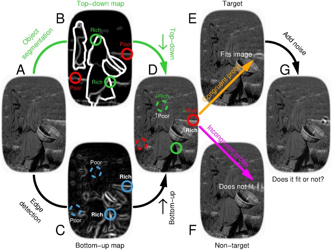
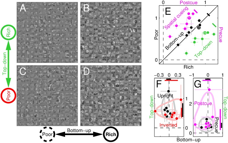
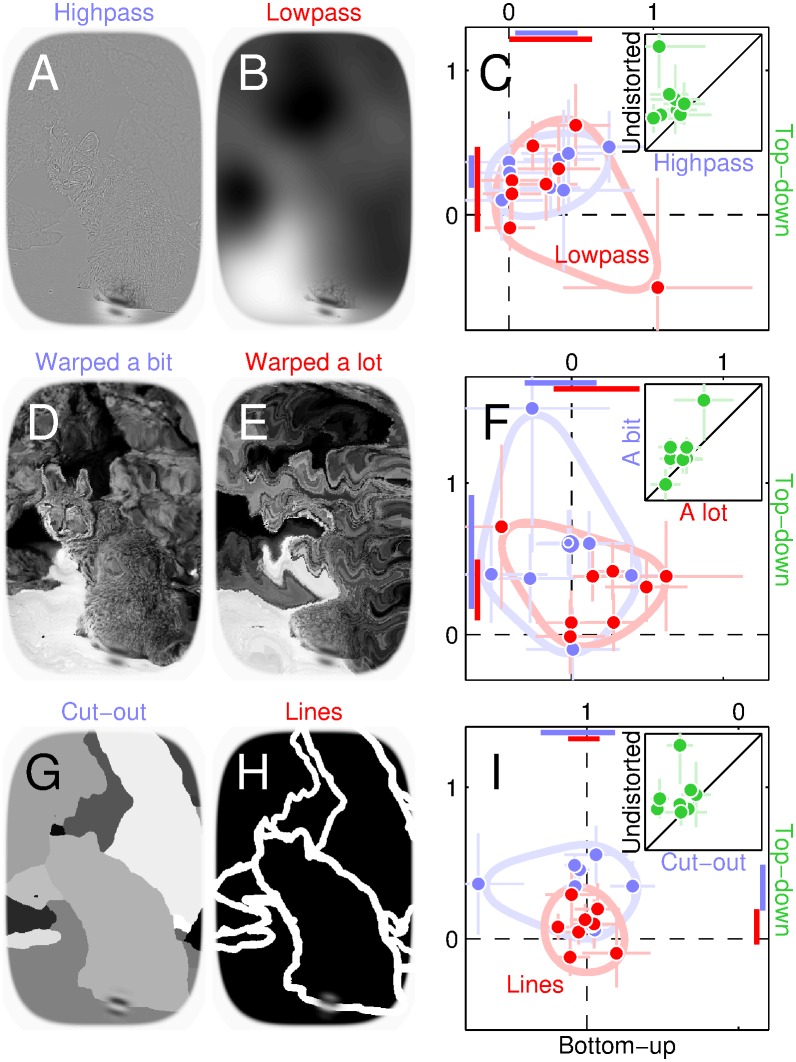
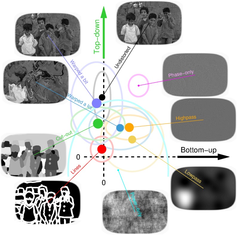
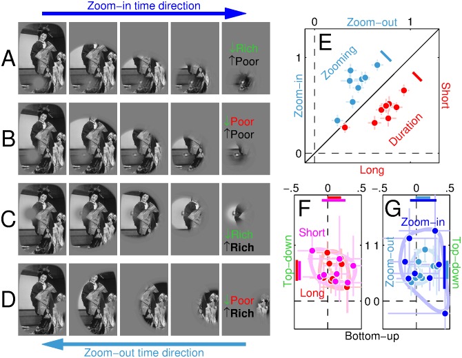
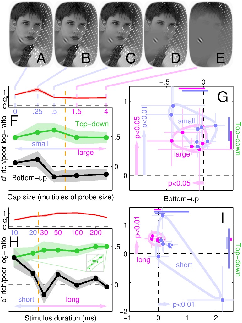
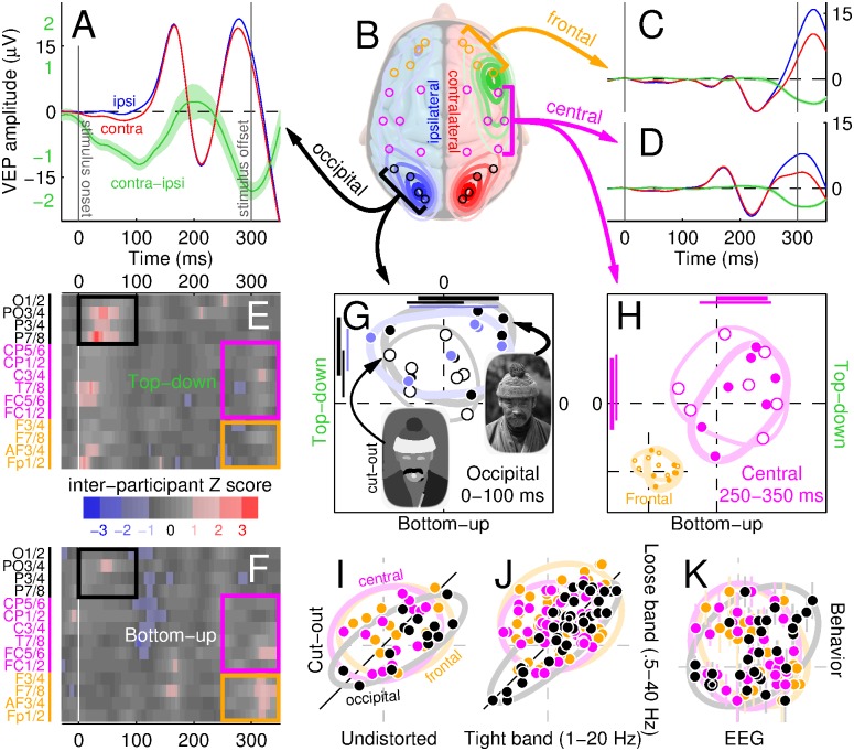
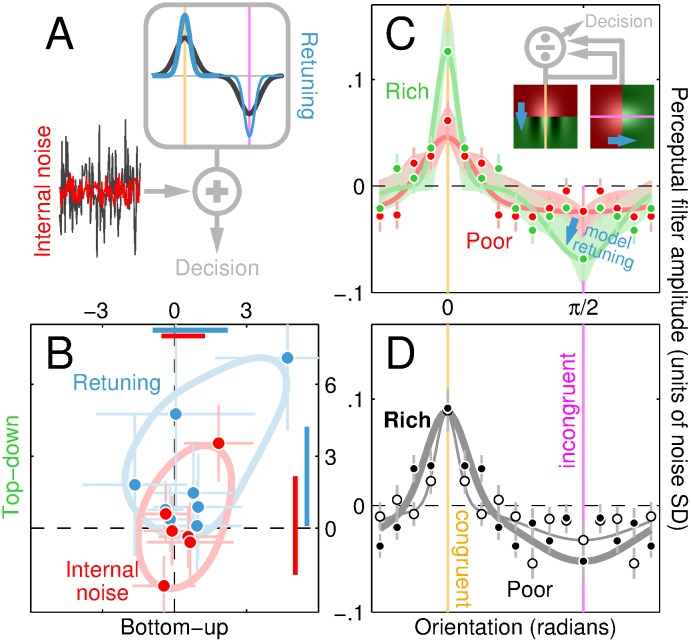
The structure of the physical world projects images onto our eyes. However, those images are often poorly representative of environmental structure: well-defined boundaries within the eye may correspond to irrelevant features of the physical world, while critical features of the physical world may be nearly invisible at the retinal projection. The challenge for the visual cortex is to sort these two types of features according to their utility in ultimately reconstructing percepts and interpreting the constituents of the scene. We describe a novel paradigm that enabled us to selectively evaluate the relative role played by these two feature classes in signal reconstruction from corrupted images. Our measurements demonstrate that this process is quickly dominated by the inferred structure of the environment, and only minimally controlled by variations of raw image content. The inferential mechanism is spatially global and its impact on early visual cortex is fast. Furthermore, it retunes local visual processing for more efficient feature extraction without altering the intrinsic transduction noise. The basic properties of this process can be partially captured by a combination of small-scale circuit models and large-scale network architectures. Taken together, our results challenge compartmentalized notions of bottom-up/top-down perception and suggest instead that these two modes are best viewed as an integrated perceptual mechanism.

Fig 1. Mapping features from natural scenes.

Intensity (brightness) on the top-down map (B) reflects saliency of perceptual object representation within the original scene [5, 6] (A), while the bottom-up map (C) indicates edge energy content [3, 7]. We identify 4 locations that are rich/poor on the top-down map (green/red circles in B) and/or rich/poor on the bottom-up map (solid/dashed circles in C); the two locations indicated by dashed-green and solid-red circles in D are rich on one map and poor on the other. An oriented wavelet is inserted at one location in congruent (E) or incongruent (F) configuration, orientation noise is added [8] (G), and observers must determine whether probe is congruent or not [9, 10].

Fig 2. Performance is driven by top-down map.

A-D show collections of image regions (approximately 3 × probe size) surrounding probe insertion points (with embedded congruent probe) at rich/poor locations on top-down map (A-B versus C-D) or bottom-up map (B,D versus A,C). The poor→rich transition is perceptually evident across the bottom-up map (left → right). E plots sensitivity (d′) for poor (y axis) versus rich (x axis) locations on the bottom-up (black) or top-down map (green) in individual observers (1 symbol per observer), as well as precue (y axis) versus postcue (x axis) configurations (magenta). F-G plot sensitivity rich/poor log-ratios for top-down (y axis) and bottom-up (x axis) comparisons when scenes were upright or inverted (black or red in F) and precued or postcued (black or magenta in G). Error bars plot ±1 SEM. Coloured diagonal segments in E plot 95% confidence intervals for data projected along negative diagonal. Horizontal/vertical segments near x/y axes in F-G plot confidence intervals for bottom-up/top-down log-ratio effects; light-coloured contours indicate data spread for visualization aid. Data for this figure is available from S2 Data.

Fig 3. Scene manipulations may eliminate top-down effects and/or produce bottom-up effects.

Natural scenes were highpass/lowpass filtered (A-B), warped a bit or a lot (D-E), and converted to cut-out or line versions (G-H). C,F,I are plotted to the conventions adopted in Fig 2F and 2G; insets plot top-down effects for specific comparisons. Data for this figure is available from S2 Data.

Fig 4. Summary of image manipulations.

Top-down (y axis) and bottom-up (x axis) effects are plotted for all scene manipulations averaged across observers (each symbol shows average for the indicated configuration, ovals plot ±1 SD across observers). Symbol size scales with absolute efficiency [35] (directly proportional to d′ and inversely proportional to stimulus SNR). Data for this figure is available from S2 Data.

Fig 5. Scene-probe dynamics impacts absolute sensitivity but not differential effects.

Zooming stimuli involve smooth transitions from scenes without probes (leftmost icons in A-D) to probes without scenes (rightmost icons) in either scene-to-probe “zoom-in” direction (left to right in A-D) or probe-to-scene “zoom-out” direction (right to left). E plots sensitivity (d′) for zoom-in (y axis) versus zoom-out (x axis) configurations (blue symbols) and long-duration (300 ms, x axis) versus short-duration (100 ms, y axis) stimuli (red) using conventions similar to Fig 2E. F-G plot corresponding log-ratios using conventions similar to Fig 2F and 2G. Data for this figure is available from S2 Data.

Fig 6. Top-down effect is spatially global (F) but reduced at ultrashort durations (H).

F plots d′ log-ratios for bottom-up (black) and top-down (green) effects as a function of gap size (x axis) for spatial gaps of differing size between probe and scene (A-E), pooled across observers. Red trace plots overall d′. Shading shows ±1 SEM. G plots log-ratios for individual observers (conventions similar to Fig 2F) pooled separately from small (gap < probe, blue) and large (gap > probe, magenta) gap sizes. H-I show similar measurements for varying stimulus durations, short (< 30 ms, blue) and long (≥30 ms, magenta). Inset to H replots green data with rescaled y axis to emphasize positive trend (solid line shows best linear fit, dashed lines 95% confidence intervals for fit). Vertical/horizontal arrows in G,I point to average y/x values for effects associated with significant p-values (<0.05) from Wilcoxon signed-rank test for different than 0 (p-values are indicated next to arrow). Thin blue segments near axes in I show confidence intervals for blue dataset after removal of data point at bottom-right of panel. Data for this figure is available from S2 Data.

Fig 7. Top-down effects operate quickly within occipital cortex.

A,C,D plot evoked potentials from occipital, central, and frontal electrodes marked by black, magenta, and orange circles in B. Blue/red trace shows waveform from electrodes ipsilateral/contralateral to probe location; green trace shows contralateral-minus-ipsilateral difference (shading shows ±2 SEM). Contour plots in B show interpolated scalp distribution of potential RMS for ipsilateral/contralateral waveforms (blue/red), as well as the ratio between contra-minus-ipsi waveform RMS and overall (ipsi + contra) RMS (green). E-F show the difference between rich and poor probe insertions for contra-minus-ipsi vaweform with respect to top-down (E) and bottom-up (F) maps, separately for the different electrodes (indexed on the y axis as pairs from which individual rows were computed), in the form of Z scores across participants. G plots RMS-normalized modulations (see Methods) in E/F on y/x axes pooled within black rectangles (occipital electrodes) in E/F, separately for different participants (1 symbol per participant, conventions similar to Fig 2F); solid symbols refer to intact scenes, open symbols to cut-out variant, blue symbols to results following artefact rejection (see Methods). H plots similar results from modulations pooled within magenta rectangles (central electrodes) in E/F; inset to H from modulations within orange rectangles (frontal electrodes). I-K plot the pooled quantities in G-H for specific comparisons on x- versus y-axes (top-down and bottom-up values are collated without distinction for this analysis): intact (undistorted) scenes versus cut-out variant (I); highpass/lowpass filtering of 1/20 Hz versus 0.5/40 Hz (J); values for intact scenes versus d′ log-ratios from Fig 2F (K). Ovals in I-K are aligned with best-fit line, with axes matched to 2 SD for values projected onto axes parallel/orthogonal to line. Data for this figure is available from S2 Data. EEG, electroencephalogram; RMS, root-mean-square; VEP, visual evoked potential.

Fig 8. Top-down enhancement is driven by sensory retuning.

A sketches minimal SDT model consisting of front-end filter (grey box) followed by additive internal noise (black random trace pointing to + symbol); sensitivity may be enhanced by reducing internal noise (red trace), sharpening filter around congruent (thick blue line) and/or incongruent orientation (thin blue line). B plots rich/poor log-ratios for internal noise estimates (red) and projected sensitivity from filter estimates (blue) returned by psychophysical reverse correlation (plotting conventions similar to Fig 2F). Aggregate perceptual filters are shown in C-D for rich vs poor locations on top-down (C, green versus red) and bottom-up (D, solid versus open) maps. Congruent/incongruent orientations are indicated by orange/magenta vertical lines (0 and π/2 on x axis). Error bars show ±1 SEM. Lines show fits from 2 Gaussian functions of opposite sign centred on congruent/incongruent orientations (for visualization only). Shading in C plots ±1 SD across simulations from gain-control model (inset), consisting of 2 front-end filters oriented along congruent (left icon in inset) and incongruent (right icon) orientations. Model simulations for red/green shading were generated by red/green-tinted front-end filters (transition indicated by blue arrows). Data for this figure is available from S2 Data. SDT, signal detection theory.

Fig 9. Deep networks generate good proxy for top-down representation.

A-C plot human sensitivity (y axis) for individual probe insertions (one small dot per insertion) separately for different scenes (pooled across participants), against values corresponding to probe insertion point on top-down/bottom-up maps (A/B) and the map generated by the CRF-RNN deep convolutional network [23] (C; abscissa values for this plot have been rescaled to range between 0 and 1). Dashed lines show 80%, 90%, and 95% (from thick to thin) confidence intervals for linear fit. Green symbols in A show average y value for individual abscissa values; symbol size scales with number of data points. D shows correlation values for scatter plots in A-C and those generated by other computer vision algorithms (Itti-Koch [3], GBVS [41], gPb-HS [5], nCuts [42], HVC [43]); open green symbol plots correlation for top-down map when consensus probe locations (indicated by solid green symbol in A) are excluded. Error bars in D show 95% confidence intervals. E plots rich/poor log-ratios to the conventions of Fig 2F where human sensitivity estimation for y axis is relabelled against rich/poor probe locations on the maps generated by CRF-RNN (red) and gPb-HS (blue) algorithms instead of top-down map (black). Values on the x axis are computed with respect to bottom-up map (same as Fig 2F). Icons show example segmentations from the two algorithms for the natural scene in Fig 1A; coloured overlay indicates segmented regions/boundaries, orange circle corresponds to red solid circle (top-down poor, bottom-up rich location) in Fig 1D. Data for this figure is available from S2 Data. HVC, hierarchical visual cues; GBVS, graph-based visual saliency.

References

1. Hubel DH. The visual cortex of the brain. Sci Am. 1963;209:54–62. - PubMed
1. Marr DC. Vision: A Computational Investigation into the Human Representation and Processing of Visual Information. New York: Freeman; 1982.
1. Itti L, Koch C. Computational modelling of visual attention. Nat Rev Neurosci. 2001;2(3):194–203. doi: 10.1038/35058500 - DOI - PubMed
1. Morgan MJ. Features and the 'primal sketch'. Vision Res. 2011;51:738–753. doi: 10.1016/j.visres.2010.08.002 - DOI - PMC - PubMed
1. Arbelaez P, Maire M, Fowlkes C, Malik J. Contour Detection and Hierarchical Image Segmentation. IEEE Trans Patt Anal Mach Intell. 2011;33(5):898–916. doi: 10.1109/TPAMI.2010.161 - DOI - PubMed
Publication types
LinkOut - more resources