Assessment of model accuracy estimations in CASP12

Abstract

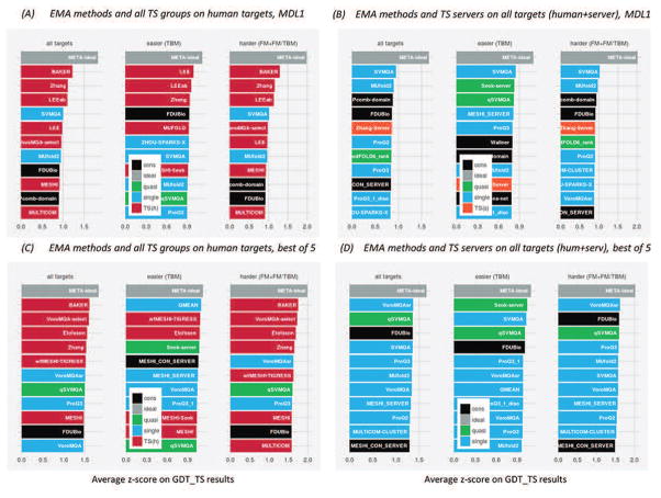
The record high 42 model accuracy estimation methods were tested in CASP12. The paper presents results of the assessment of these methods in the whole-model and per-residue accuracy modes. Scores from four different model evaluation packages were used as the "ground truth" for assessing accuracy of methods' estimates. They include a rigid-body score-GDT_TS, and three local-structure based scores-LDDT, CAD and SphereGrinder. The ability of methods to identify best models from among several available, predict model's absolute accuracy score, distinguish between good and bad models, predict accuracy of the coordinate error self-estimates, and discriminate between reliable and unreliable regions in the models was assessed. Single-model methods advanced to the point where they are better than clustering methods in picking the best models from decoy sets. On the other hand, consensus methods, taking advantage of the availability of large number of models for the same target protein, are still better in distinguishing between good and bad models and predicting local accuracy of models. The best accuracy estimation methods were shown to perform better with respect to the frozen in time reference clustering method and the results of the best method in the corresponding class of methods from the previous CASP. Top performing single-model methods were shown to do better than all but three CASP12 tertiary structure predictors when evaluated as model selectors.

Keywords: CASP; EMA; QA; estimation of model accuracy; model quality assessment; protein structure modeling; protein structure prediction.

Figure 1

Average difference in global accuracy estimates submitted by CASP12 predictors on the same models in two different stages of the EMA experiment. Groups are sorted by the increasing average absolute difference between the stage 1 and stage 2 scores. The red horizontal line (corresponding to a difference of 0.02) separates methods that generate approximately the same accuracy scores for the same models in both stages of the experiment (above) and those that do not (below). Single-model methods (blue) and clustering methods (black) are on different sides of the line. Quasi-single methods (green) can be found on both sides of the separation line.

Figure 2

Ability of CASP12 accuracy estimate methods to select the best model in decoy sets. (A) Average difference in accuracy between the models predicted to be the best and the actual best according to the GDT_TS score. For each group, the differences are averaged over all predicted targets for which at least one structural model had a GDT_TS score above 40. Clustering methods are in black, single-model methods in blue, and quasi-single model methods in green. Lower scores indicate better group performance. (B) A summary of the “best selector” results expressed as the cumulative ranking of the participating methods according to four evaluation scores –GDT_TS (yellow), CADaa (red), SphereGrinder (dark red) and LDDT (orange). Single-model methods are in leading roles with the ProQ3 and SVMQA ranked in the top two according to all evaluation measures.

Figure 3

Success rates of CASP12 methods in identifying best models. (A) The percentage of targets where the best EMA model is less than 2 (green bars), more than 2 and less than 10 (yellow), and more than 10 (red) GDT_TS units away from the actual best model. The percentages are calculated on targets for which at least one structural model had a GDT_TS score above 40. Groups are sorted by the difference between the rates of successful and failed predictions (green and red bars). Top performing groups can correctly identify the best models in approximately 40% of the test cases. (B) Cumulative ranking of the groups based on the differences between their success and failure rates calculated with GDT_TS, LDDT, CADaa, and SphereGrinder measures. Method coloring scheme is the same as in Figure 2.

Figure 4

(A) Accuracy estimates as compared to the GDT_TS scores of the assessed models. For each group, deviations are calculated for each model and then averaged over all predicted models. Group name colors in the plot distinguish different types of methods: clustering methods are in black, single-model in blue, and quasi-single in green. Lower scores indicate better group performance. The best performing methods are capable of predicting the absolute accuracy of models with an average per-target error of 5 GDT_TS. (B) Cumulative ranking of methods by the deviations of absolute accuracy estimates according to four evaluation measures - GDT_TS, LDDT, CADaa, and SphereGrinder. Method coloring scheme is the same as in Figure 2. Three quasi-single methods are leading the cumulative ranking.

Figure 5

Ability of methods to discriminate between good and bad models. (A) ROC curves for top 10 EMA groups on the GDT_TS data. The separation threshold between good and bad models is set to GDT_TS=50. Groups are ordered according to decreasing AUC score, which is provided in the legend after the group name. For clarity, only the left upper part of the ROC-curve graph is shown (FPR≤0.3, TPR≥0.7). (B) Cumulative ranking of groups based on the AUCs calculated on the GDT_TS, LDDT, CADaa and SphereGrinder data. Method coloring scheme is the same as in Figure 2. Clustering methods demonstrate dominance in this aspect of analysis.

Figure 6

Average ASE score calculated on (A) whole targets and (B) structural subdomains. Results in both evaluation modes are very similar, with the best methods exceeding ASE=80.

Figure 7

Accuracy of the binary classifications of residues (reliable/unreliable) based on the results of the ROC analysis on whole targets. (A) ROC curves for top 12 EMA groups on the distance error data. A residue in a model is defined to be correct when its Cα is within 3.8Å from the corresponding residue in the target. Group names are ordered according to decreasing AUC scores, which are provided in the legend in parentheses. For clarity, only the left upper quadrant of a typical ROC-plot is shown (FPR≤0.5, TPR≥0.5). (B) AUC values for all participating groups. Clustering methods demonstrate better results, but cannot outperform the reference Davis-EMAconsensus method.

Figure 8

Relative scores of the best overall methods (red) and single-model methods (blue) in CASP12 (dark color) and CASP11 (light color). The first three scores along the x-axis are based on comparison of the GDT_TS scores in the QAglob analysis (sections 2.1–2.3 in the text), the last two – on comparison of the distance errors in the QAloc analysis (sections 3.1.–3.2). For each of the five selected measures, the ratio between the score of the best participating method (overall or single-model) and the score of the Davis-EMAconsensus method is calculated. Two ratios - average deviation and loss from the best - are inverted so that higher bars in the graph always indicate a better result. Values above 1.0 mean that the best method outperforms the baseline method. Single-model methods in CASP12 demonstrate improved performance across the board.

Figure 9

Comparison of the EMA methods with the tertiary structure prediction methods according to GDT_TS. Panels A and B show the data for first models, while panels C and D for best-out-of-five models. (A, C) Joined ranking of the EMA methods and all TS groups on human targets; (B, D) Joined ranking of the EMA methods and server TS groups on all targets. Rankings are provided separately for all targets, easier targets (TBM) and harder targets (FM and FM/TBM targets). Model accuracy estimation methods are colored as in the rest of the paper: single-model methods in blue, quasi-single in green, and clustering in black; tertiary structure prediction methods are colored as follows: human-expert groups in red, servers in orange. All graphs include the data for the perfect meta-predictor, which always picks the best server model (META-ideal, grey). EMA methods rival performance of the best TS methods in all target difficulty categories, with the perfect meta-predictor being consistently on top of rankings.

Figure 10

Cumulative ranking of the EMA methods and the tertiary structure prediction methods on the first models according to four evaluation scores – GDT_TS (yellow), LDDT (orange), CADaa (red), and SphereGrinder (dark red). The best 20 methods in joined ranking are shown. Method coloring scheme is the same as in Figure 9. Being assessed as tertiary structure meta-predictors, accuracy assessment methods rival best expert groups and outperform CASP servers.

Figure 11

Boxplots showing per-target distribution of the actual accuracy of server models in the best150 dataset (150 model-target GDT_TS scores, panel A), similarity of models in the best 150 dataset (150*149=22350 model-model pairwise GDT_TS scores, panel B), and the accuracy estimates from the top 5 clustering methods (panel C), quasi-single methods (panel D) and single-model methods (panel E). Each of the panels (C–E) contains 150 data points representing average EMA scores from the selected five methods on a particular target. Box boundaries correspond to the25th (bottom) and 75th (top) percentiles in the data; the horizontal line inside the box corresponds to the median. The height of the box defines the interquartile range (IQR). The height of the whiskers shows the range of values outside the interquartile range, but within 1.5 IQR. The black dots correspond to the outliers outside the 1.5 IQR range. Targets are sorted by the descending median GDT_TS score of the model set (panel A). Single-domain targets are marked with the letter (S) next to the target number, multi-domain with letter (M).

Figure 12

Deviation between the predicted (EMA) and actual (GDT_TS) scores of server models in the best150 dataset, as a function of (A) target difficulty represented by the median GDT_TS score and (B) similarity of models represented by the per-target interquartile width of the pairwise model-model GDT_TS scores. Each point corresponds to one target. For each target and each EMA group, absolute deviations are calculated for every TS model and then averaged over all predicted models. The minimum average deviation among all EMA groups submitting on the target is plotted with the color corresponding to the type of the best performing method (blue for single, green for quasi-single and black for clustering). Ties are resolved in the order: single, quasi-single, clustering. Lower scores indicate better predicted targets. Black lines run visibly lower than blue and green ones, indicating advantage of clustering methods over single and quasi-single methods in this aspect of analysis. Targets T0862 and T0866 are among the most challenging for predicting absolute accuracy scores, while T0867 is an example of target with very good EMA predictions.

Figure 13

Difference in accuracy of models predicted to be the best and the actual best according to the GDT_TS score as a function of the separation between the best model and the distribution mean (GDT_TS-based z-score). Each point corresponds to one target. The data are shown for targets with at least one structural model scoring GDT_TS>40. For each target, the minimum deviation among all EMA groups is plotted, with the color corresponding to the type of the best performing method (blue for single, green for quasi-single and black for clustering). Ties are resolved in the order: single, quasi-single, clustering. Lower scores indicate better predicted targets. Larger slope of the line indicates larger dependency of the methods on the separation between the best model and the mean model in terms of the GDT_TS score. Targets T0890, T0900 and T0942 are examples of the largest failures. Targets T0868, T0884, T0866 and T0885 are all examples of the successful identification of best models on the targets where only few models were much better than the others.

References

1. Kryshtafovych A, Barbato A, Monastyrskyy B, Fidelis K, Schwede T, Tramontano A. Methods of model accuracy estimation can help selecting the best models from decoy sets: Assessment of model accuracy estimations in CASP11. Proteins. 2016;84(Suppl 1):349–369. - PMC - PubMed
1. Kryshtafovych A, Barbato A, Fidelis K, Monastyrskyy B, Schwede T, Tramontano A. Assessment of the assessment: evaluation of the model quality estimates in CASP10. Proteins. 2014;82(Suppl 2):112–126. - PMC - PubMed
1. Kryshtafovych A, Fidelis K, Tramontano A. Evaluation of model quality predictions in CASP9. Proteins. 2011;79(Suppl 10):91–106. - PMC - PubMed
1. Cozzetto D, Kryshtafovych A, Tramontano A. Evaluation of CASP8 model quality predictions. Proteins. 2009;77(Suppl 9):157–166. - PubMed
1. Cozzetto D, Kryshtafovych A, Ceriani M, Tramontano A. Assessment of predictions in the model quality assessment category. Proteins. 2007;69(Suppl 8):175–183. - PubMed
Publication types