The divisive normalization model of V1 neurons: a comprehensive comparison of physiological data and model predictions

Abstract

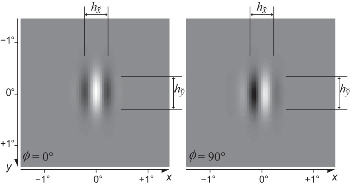
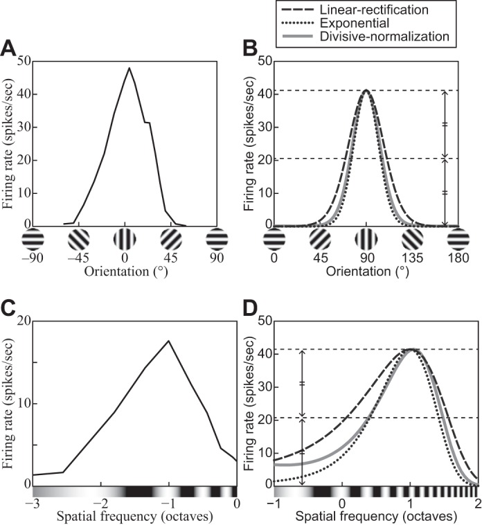
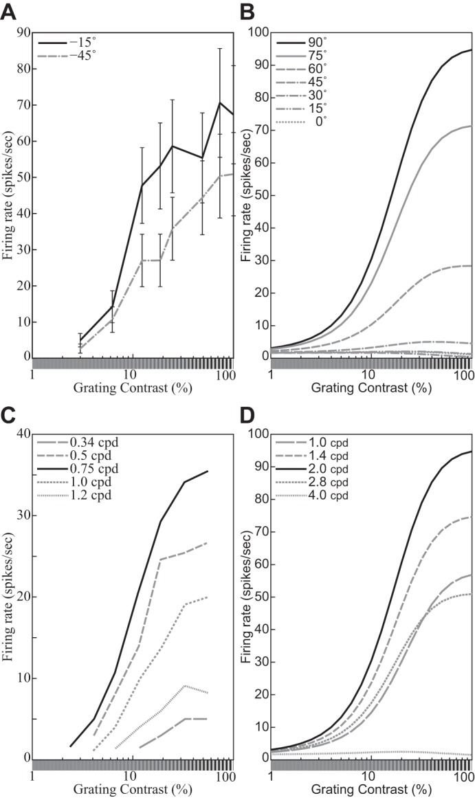
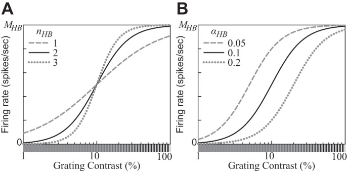
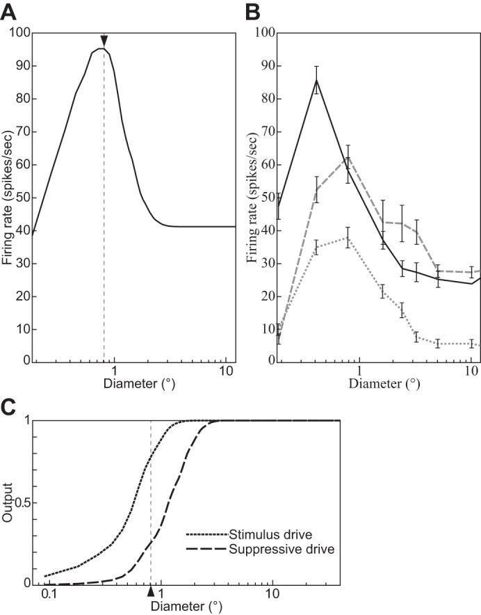
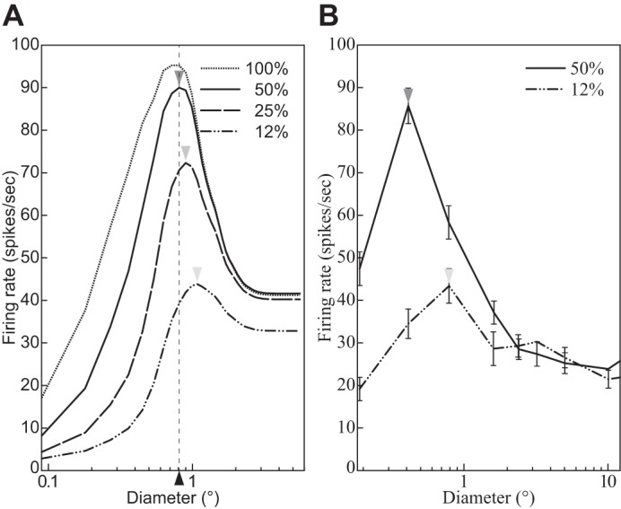
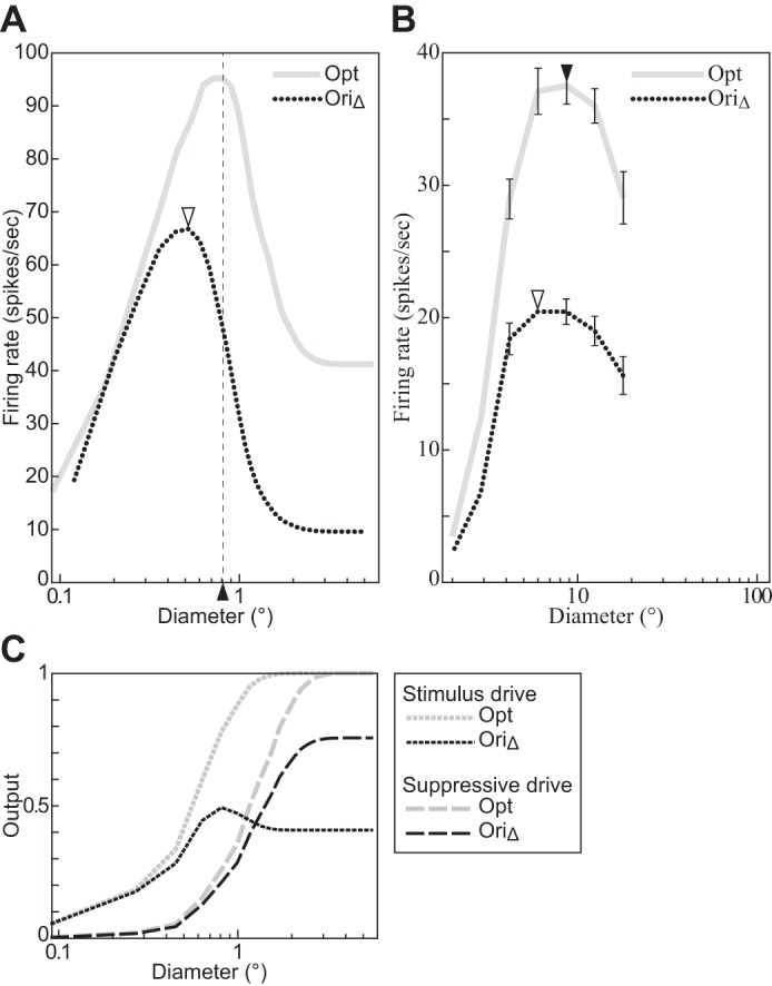
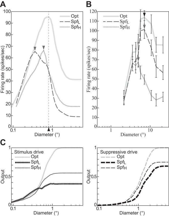
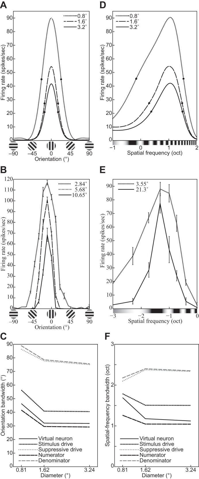
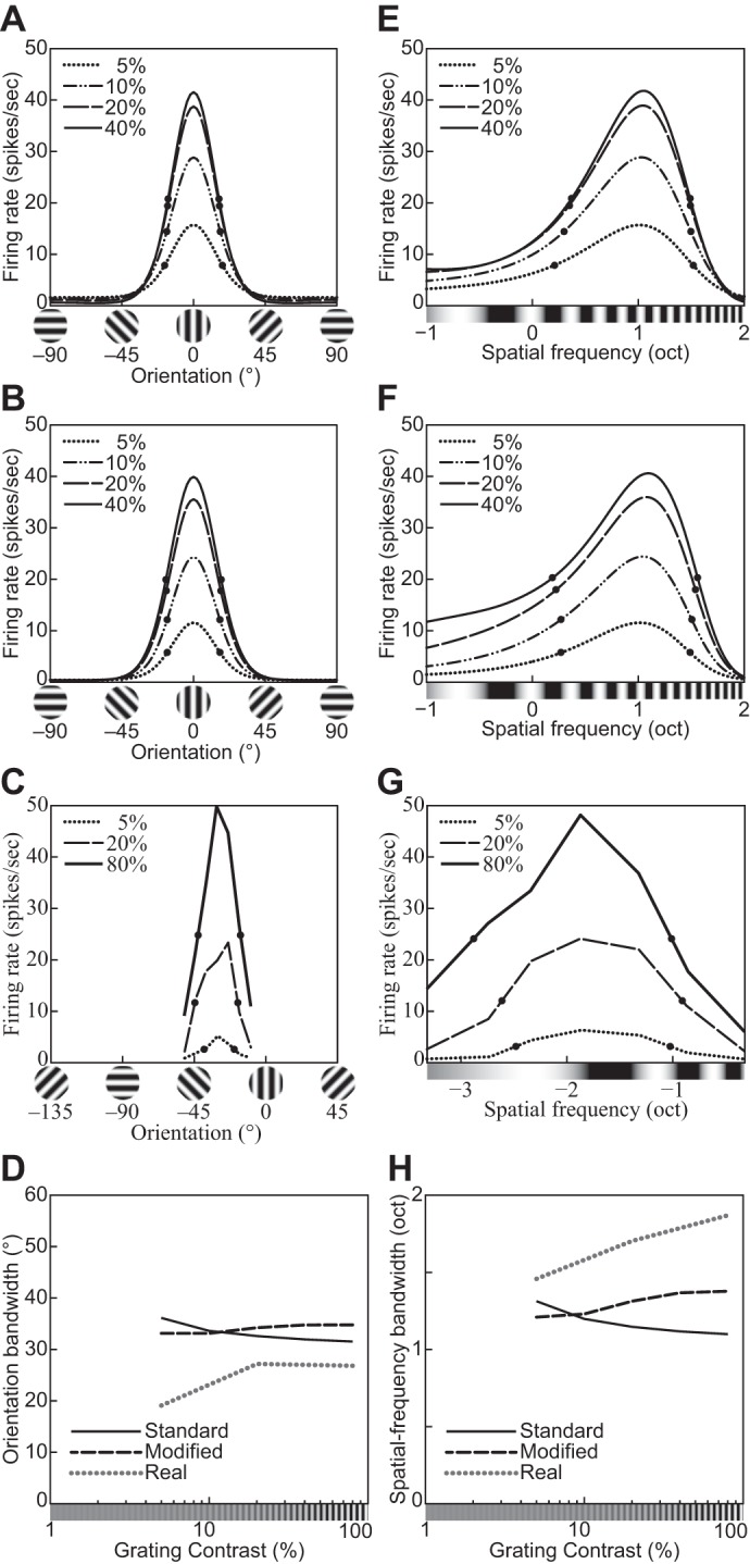
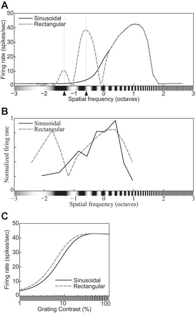
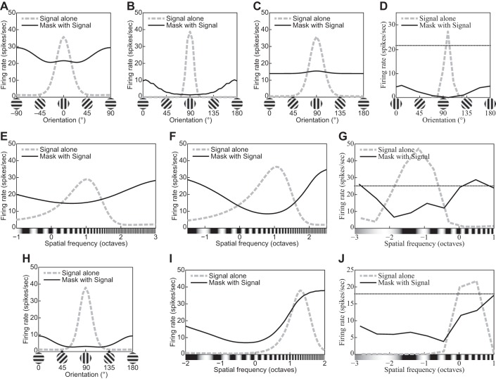
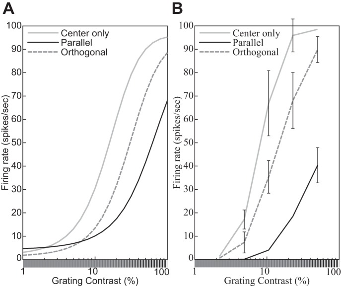
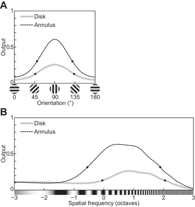
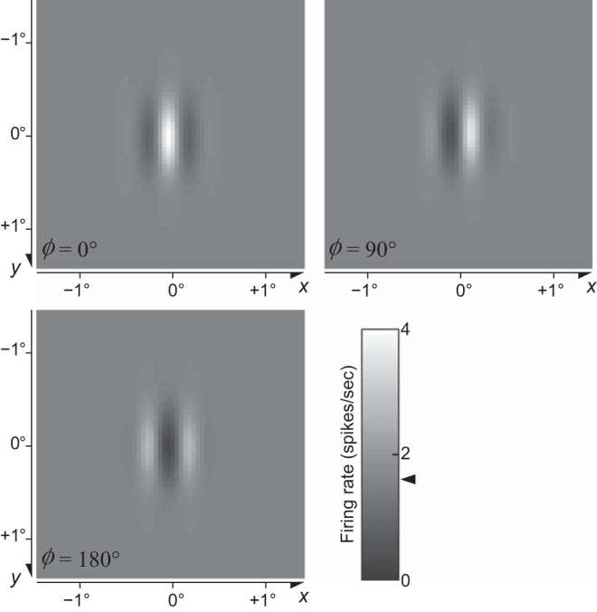
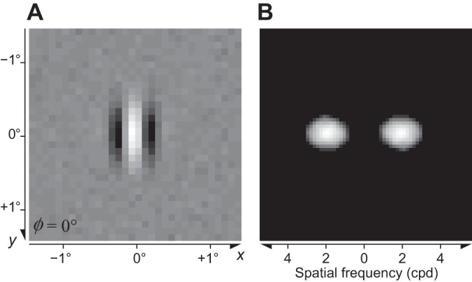
The physiological responses of simple and complex cells in the primary visual cortex (V1) have been studied extensively and modeled at different levels. At the functional level, the divisive normalization model (DNM; Heeger DJ. Vis Neurosci 9: 181-197, 1992) has accounted for a wide range of single-cell recordings in terms of a combination of linear filtering, nonlinear rectification, and divisive normalization. We propose standardizing the formulation of the DNM and implementing it in software that takes static grayscale images as inputs and produces firing rate responses as outputs. We also review a comprehensive suite of 30 empirical phenomena and report a series of simulation experiments that qualitatively replicate dozens of key experiments with a standard parameter set consistent with physiological measurements. This systematic approach identifies novel falsifiable predictions of the DNM. We show how the model simultaneously satisfies the conflicting desiderata of flexibility and falsifiability. Our key idea is that, while adjustable parameters are needed to accommodate the diversity across neurons, they must be fixed for a given individual neuron. This requirement introduces falsifiable constraints when this single neuron is probed with multiple stimuli. We also present mathematical analyses and simulation experiments that explicate some of these constraints.

Keywords: complex cells; computational modeling; divisive normalization; primary visual cortex (V1); simple cells.

Fig. 1.

Examples of Gabor patches with phase Φ = 0° and Φ = 90°, vertical orientation (Θ = 0°), and spatial frequency F = 2 cpd (Eq. 2). The parameters $h_{\breve{x}}$ and $h_{\breve{y}}$ control the full width at half height (FWHH) of the Gaussian envelope along the directions that are perpendicular and parallel to the grating, respectively.

Fig. 2.

A: a representative orientation tuning curve—in this case from a V1 complex cell of an anesthetized cat. Replotted from Fig. 1 in Rose and Blakemore (1974). B: orientation tuning curves of 3 models introduced in the main text: linear rectification (Eq. 6), exponential (Eq. 11), and divisive normalization (DNM, Eq. 15). Each model neuron was probed with gratings with 100% contrast, 5.76° size, and the neuron’s preferred phase and frequency. All 3 models used the same weighting function for the linear filtering stage and DNM’s standard bandwidth parameters (see Standard parameter set). The stimulus drive exponent of the exponential model (n_Ex = n_n = 2) was set to its counterpart in the standard DNM parameter set (Table 2). C: a representative spatial-frequency tuning curve—in this case from a V1 simple cell of an anesthetized cat. Replotted from Li and Li (1994, Fig. 7C). D: spatial-frequency tuning curves of the 3 models described in C. The grating probes had 100% contrast, 5.76° size, and the neuron’s preferred phase and orientation. Dotted lines depict the full and half heights of the curves. (See phenomena 13 and 14 in Table 1.)

Fig. 3.

Representative contrast response functions (CFs). A: responses of a simple cell to drifting sinusoidal gratings spanning a range of contrasts at 2 orientations (see key). Replotted from Carandini et al. (1997, Fig. 4B, anesthetized macaque; error bars =  ±SE). B: CFs of the DNM neuron with default parameters, probed with gratings with the neuron’s preferred frequency (1.0 oct) and orientations shown in key. The size of the stimuli was equal to the measured RF diameter (0.81°). C: responses of a V1 neuron to drifting sinusoidal gratings with the neuron’s preferred orientation and spatial frequencies shown in key. Replotted from Albrecht and Hamilton (1982, Fig. 7A). D: CFs of the divisive normalization model (DNM, defined in text) neuron with default parameters, probed with gratings with the neuron’s preferred orientation (0°) and spatial frequencies shown in key. The size of the stimuli was equal to the measured RF diameter (0.81°). (See phenomena 7, 10, and 11 in Table 1.)

Fig. 4.

Contrast response functions (CFs) produced by the hyperbolic ratio model (Eq. 12). A: the exponent parameter n_HB controls the slope of the CF as a function of the log contrast of the stimulus. B: the semisaturation contrast parameter α_HB controls the location of the CF. A stimulus with contrast α_HB elicits one-half of the saturation level M_HB. (α_HB = 0.1 for A; n_HB = 2 for B.)

Fig. 5.

Size tuning functions of a divisive normalization model (DNM) complex cell with standard parameters (A), 3 V1 complex cells (B) (replotted from Schwabe et al. 2010, Fig. 2, anesthetized macaque; error bars =  ±SE), and the stimulus and suppressive drive terms of the DNM equation (C). The measured RF diameter of the DNM neuron is 0.81° (indicated by arrowhead in A). All stimuli were gratings with maximal contrast (c = 1) and orientation and frequency that matched the preferences of the respective neuron. (See phenomenon 1 in Table 1.)

Fig. 6.

The size tuning function depends on the contrast of the stimulus grating. A: divisive normalization model (DNM) complex cell with standard parameters. B: V1 complex cell (replotted from Schwabe et al. 2010, Fig. 2a, anesthetized macaque; error bars =  ±SE). The measured RF diameter (depicted by arrowheads) increases as the stimulus contrast (shown in key) decreases. Stimulus orientation and frequency matched the preferences of the respective neuron. (See phenomenon 2 in Table 1).

Fig. 7.

The size tuning function depends on the orientation of the stimulus grating. A: divisive normalization model (DNM) complex cell with standard parameters. B: V1 complex cell (replotted from Tailby et al. 2007, Fig. 2b, anesthetized cat; error bars =  ±SE). C: the stimulus and suppressive drive terms of the DNM equation. The grating orientation in the Opt condition matched the preferences of the respective neuron. The orientation in the Ori_Δ condition was determined by the half-height point of the orientation tuning function (Tailby et al. 2007). See text for details. All gratings had maximal contrast (c = 1), and their frequency matched the preference of the respective neuron. (See phenomenon 3 in Table 1.)

Fig. 8.

The size tuning function depends on the spatial frequency of the stimulus grating. A: divisive normalization model (DNM) complex cell with standard parameters. B: a real V1 neuron (replotted from Osaki et al. 2011, Figs. 2A and 4A, anesthetized cat; error bars =  ±SE). C: the stimulus and suppressive drive terms of the DNM equation. The stimulus frequency matched the preference of the respective neuron in the Opt condition, was lower in the Spf_L condition, and was higher in the Spf_H condition. The side frequencies in A were determined by the half-height points of the DNM frequency tuning curve. See text for details. The data in B were collected with Spf_L = 0.10 cpd, Opt = 0.20 cpd, and Spf_H = 0.30 cpd (Osaki et al. 2011). All gratings had maximal contrast (c = 1), and their orientation matched the preference of the respective neuron. (See phenomenon 4 in Table 1.)

Fig. 9.

Responses to annular stimuli containing a circular gray “hole” inside a large circular grating. x-Axis specifies the diameter of the hole for annular stimuli and the outside diameter for disk stimuli (cf. Fig. 5). A: DNM complex cell with standard parameters. Key indicates the contrast of the annular stimuli; the disk had 100% contrast. The measured RF diameter (0.81°) is indicated by arrowhead. B: V1 neuron for which the 2 operational procedures yield comparable diameters (replotted from Jones et al. 2001, Fig. 1, anesthetized macaque; error bars =  ±SE). C: DNM complex cell with a modified parameter set (M = 25, n_d = 2.5, β = 0.005, α = 0.04). Both disk and annulus had 100% contrast. The measured RF diameter (0.36°) is indicated by vertical dashed line. D: V1 neuron for which the annulus-measured diameter is larger than the disk-measured diameter (replotted from Cavanaugh et al. 2002a, Fig. 4, anesthetized macaque). All stimuli are based on gratings whose frequency and orientation matched the preference of the respective neuron. (See phenomena 5 and 6 in Table 1.)

Fig. 10.

An example of the supersaturation effect (phenomenon 8 in Table 1). A: contrast response function of a DNM neuron with standard (solid line) and modified (n_d = 2.35, β = 0, M = 30, dashed line) parameterization. The stimulus frequency and orientation matched the DNM preferences. The size of the grating patch was 2.88°. B: contrast response function of a real neuron (replotted from Peirce 2007, Fig. 2e, anesthetized macaque).

Fig. 11.

Responses of the model neuron (A and C) and a V1 simple cell (replotted from Carandini et al. 1997, Fig. 14, D and C, anesthetized macaque; error bars =  ±SE) (B and D) to a grating with a random noise pattern superimposed. The graphs in A and B are plotted against the contrast of the grating, whereas those in C and D are plotted against the contrast of the noise. A and C: the size of the stimuli was equal to the measured RF diameter (0.81°), and orientation and frequency matched the tuning preferences of the model neuron. (See phenomenon 9 in Table 1.)

Fig. 12.

Contrast response functions of the model neuron for gratings with different diameters (indicated in key). The contrast, orientation, and spatial frequency of the grating were 100%, 0°, and 2.0 cpd. (See phenomenon 12 in Table 1.)

Fig. 13.

Orientation and spatial-frequency tuning functions of the divisive normalization model (DNM) neuron with standard parameters (A and D), a V1 neuron (replotted from Okamoto et al. 2009, Fig. 1, anesthetized cat; error bars =  ± SE) (B), and a V1 simple cell (replotted from Osaki et al. 2011, Fig. 5B, anesthetized cat; error bars =  ± SE) (E) for gratings with different diameters (indicated in key). C and F: effect of stimulus size on the bandwidths of the DNM neuron, the numerator and denominator in Eq. 15, the stimulus drive (Eq. 9), and the suppressive drive (Eq. 18). The contrast of the grating was 100% for A and D, its frequency was 2.0 cpd for A, and its orientation was 0° for D. The full widths at half height are indicated by pairs of bold dots in A and D. (See phenomena 15 and 16 in Table 1).

Fig. 14.

Orientation and spatial-frequency tuning functions for gratings with different contrasts (indicated in key). A and E: the divisive normalization model (DNM) neuron with the standard parameter set. B and F: the DNM neuron with a modified parameter set (h_Θ = 40°, h_F = 1.0 oct). C: orientation tuning of a simple striate cell (replotted from Skottun et al. 1987, Fig. 3A, anesthetized cat). G: frequency tuning of a simple striate cell (replotted from Skottun et al. 1987, Fig. 4A, anesthetized cat). D and H: effect of stimulus contrast on the bandwidths of the real neurons in C and G and of the DNM neuron in the orientation (D) and frequency (H) domains for the 2 parameter sets (key). A, B, E, and F: the size of the grating patch was 2.88°. The spatial frequency of the grating was 2.0 cpd for A and B, and its orientation was 0° for E and F. (See phenomena 17 and 18 in Table 1.)

Fig. 15.

Spatial-frequency tuning functions for sinusoidal and square gratings of the model neuron with a modified parameter set (h_f = 0.8, h_F = 0.4) (A) and of a complex cell (replotted from Pollen and Ronner 1982, Fig. 6E, anesthetized cat) (B). Note the secondary peak at one-third of the tuned frequency for square gratings (dashed line). C: contrast response functions of the model neuron with the modified parameter set for sinusoidal and square gratings (indicated in key). (See phenomena 19 and 20 in Table 1.)

Fig. 16.

Tuning functions of the cross-orientation suppression effect. In all panels, the dashed gray line plots the excitatory tuning function obtained with nonmasked signal gratings, whereas the solid black line plots the neuron’s response to a plaid stimulus consisting of a preferred (fixed) signal and a superimposed mask grating. The horizontal axis represents the orientation/frequency of the signal or mask, respectively. The empirical tuning functions (D, G, and J) were measured in separate sessions with different grating contrasts. The horizontal dotted lines in these graphs represent the neuron’s response to a nonmasked signal with the same contrast as the signal component of the plaids in the suppression sessions (see DeAngelis et al. 1992 for details). The cross-orientation suppression effect is the mask-induced decrement relative to this baseline. A: orientation tuning of the DNM neuron with standard parameters (signal c = 15%, mask c = 25%). B: orientation tuning of a DNM neuron with modified parameters (n_n = n_d = 10, h_Θ = 55, M = 11; signal c = 15%, mask c = 25%). C: orientation tuning of a DNM neuron with modified parameters (h_Θ = 90, h_f = 1.0; signal c = 15%, mask c = 25%). D: orientation tuning of a complex cell (replotted from DeAngelis et al. 1992, Fig. 7, C and D, anesthetized cat; signal f = 1.25, mask f = 0.6 cpd). E: frequency tuning of the DNM neuron with standard parameters (cf. A; signal c = 10%, mask c = 25%). F: frequency tuning of a DNM neuron with modified parameters (h_F = 1.0, h_Θ = 90, R = 50; signal c = 10%, mask c = 25%). G: frequency tuning of a simple cell (DeAngelis et al. 1992, Fig. 3, A and B; signal c = 10%, mask c = 25%). H and I: orientation and frequency tuning of an augmented DNM neuron that had an extra parameter μ_F so that the pooling kernel of the suppressive drive could be set independently from the preferred frequency of the stimulus drive (appendix e; μ_F = −1 oct, h_F = 1.0, α = 0.03, M = 3; signal c = 15%, mask c = 25%). Note that the preferred frequency of the augmented DNM neuron with μ_F = −1 oct is 2.46 cpd and is clearly different from the preferred frequency of the stimulus drive F* = 2.0 cpd. J: frequency tuning of the same complex cell as D (DeAngelis et al. 1992, Fig. 3, C and D; signal c = 15%, mask c = 25%). All frequency tuning functions were obtained with plaids with orthogonal signal and mask orientations. All simulated orientation tuning functions were obtained with signal f = 2, mask f = 1 cpd (except for H: signal f = 2.46, mask f = 1.23 cpd). Stimulus size was 2.88° in all simulations. (Note: signal/mask f = frequency of the respective component of a plaid, c = contrast.) (See phenomena 21 and 22 in Table 1.)

Fig. 17.

A: contrast response functions of the model neuron with standard parameters for a signal grating alone (dashed line, cf. Fig. 3) and for an orthogonal plaid composed of signal and mask gratings with equal contrasts (solid line). B: the suppression index (SI, defined in text) for the model neuron with 4 different parameter sets is plotted as a function of the contrast of either grating in an isocontrast plaid. Key indicates which parameters have been modified from their standard values (Table 2). The 2 diamonds depict the median SIs measured for 2 contrasts in a sample of 32 simple cells (Priebe and Ferster 2006, Table 1, anesthetized cat).

Fig. 18.

Effect of cross-orientation suppression on the contrast response functions of the model neuron with standard parameters (A and C) and a V1 neuron (replotted from Freeman et al. 2002, Fig. 6, anesthetized cat) (B and D). In A and B, the responses of the model and real neurons are plotted against the contrast of the signal grating, with mask contrast shown in key. In C and D, the responses are plotted against the contrast of the mask grating, with signal contrast in key. A and C: the size of the stimuli was equal to the measured RF diameter (0.81°). The orientations of the signal and mask gratings were 0° and 90°, and their spatial frequency was 2.0 cpd. (See phenomenon 23 in Table 1.)

Fig. 19.

The effect of surround suppression on the response of the model neuron with standard parameters (A and C), a V1 complex cell (replotted from Cavanaugh et al. 2002b, Fig. 2B, anesthetized macaque; error bars =  ±SE) (B), and a V1 simple cell (replotted from Li and Li 1994, Fig. 7C, anesthetized cat; error bars =  ±SE) (D) in the orientation and spatial frequency domains. In all panels, the solid line plots the neuron’s response to a composite stimulus consisting of a center grating and a surrounding annulus, whereas the dashed line plots the standard tuning function as probed with the center alone. x-Axis represents the orientation (A and B) or frequency (C and D) of the surrounding annulus for composite stimuli (solid lines) or that of the center for simple stimuli (dashed lines). A and C: the contrast of the center grating was 100%, and its diameter was 0.81° (the measured RF). The contrasts of the annulus grating were 100% and 5.76°. The frequency of the center and annular gratings was 2.0 cpd for A. Their orientation was 0° for C. (See phenomena 24 and 25 in Table 1.)

Fig. 20.

Surround-suppression effects on the contrast response functions for different contrasts of the annular grating. The contrast of the central disk is plotted on the x-axes, and the contrast of the annular surround is indicated in the key. A: the model neuron with the standard parameter set (cf. Table 2). B: a complex cell in cat V1 (replotted from Carandini 2004, Fig. 6). C: the model neuron with a modified parameter set (n_n = 2.8, n_d = 3.0, M = 10). D: a complex cell in cat V1 (replotted from Carandini 2004, Fig. 7). A and C: orientation and spatial frequency of the center and annulus gratings were 0° and 2.0 cpd. Diameter of the center grating patch was 0.81° and is equal to the measured RFs of the model neuron for both parameter sets. Size of the annulus grating was 5.76°. (See phenomenon 26 in Table 1.)

Fig. 21.

Surround-suppression effects on the contrast response functions for different orientations of the annular grating (indicated in key). A: the divisive normalization model (DNM) neuron with standard parameters. B: a simple cell (replotted from Cavanaugh et al. 2002b, Fig. 5A, anesthetized macaque; error bars =  ±SE). A: orientation of the center grating was 0°. Spatial frequency of the center and annulus gratings was 2.0 cpd. Size of the center grating patch was equal to the measured RF diameter (0.81°). Size of the annulus grating was 5.76°. (See phenomenon 27 in Table 1.)

Fig. 22.

Tuning curves of the divisive normalization model (DNM) suppressive drive term (Eq. 18) with standard parameters when probed with stimuli that are typically used to induce cross-orientation and surround suppression—a circular grating patch (Disk) and an annular grating (Annulus), respectively: orientation tuning (A) and spatial-frequency tuning (B) of the suppressive drive with respect to these 2 types of inducers. Frequency of all gratings was set to 2 cpd while measuring the orientation tuning, and their orientation was set to 0° while measuring the frequency tuning in agreement with the preferences of the DNM neuron. The diameter of Disk and the inner diameter of Annulus matched the measured receptive field diameter (0.81°). The outer diameter of Annulus was 5.76°. Compare with Fig. 16, A and E, Fig. 19, A and C, Fig. 7C, and Fig. 8C.

Fig. 23.

Receptive field maps obtained with a light spot as a probe for 3 divisive normalization model (DNM) simple cells (standard parameters) with different phases ϕ. Grayscale levels indicate firing rates. Maintained discharge (the response to a uniform gray field) was the same for the 3 cells and is indicated by arrowhead on color bar. The size of the light-spot probe was 0.045° × 0.045° (1 pixel). Stimulus background was uniform gray, and luminance of the spot was twice as high as the background gray. (See phenomenon 28 in Table 1.)

Fig. 24.

A: the receptive field of a divisive normalization model (DNM) simple cell (standard parameters) obtained via the reverse correlation method. Brighter and darker regions represent bright- and dark-excitatory regions, respectively. B: 2D Fourier spectrum energy distribution of the RF pattern in A. The stimuli were 32 × 32 mosaics of random luminance spots (white noise). Size of the stimuli was 2.88°, and that of the spots was 0.090° (2 × 2 pixels). (See phenomenon 29 in Table 1.)

Fig. 25.

A: measured 1D distributions of the responses to light and dark bars parallel to the tuned orientation of the divisive normalization model (DNM) simple cells with different phases Φ: 0° (left) and 90° (right). x-Axis represents positions of the bars along an orientation perpendicular to the tuned orientation. Top half of the graph is for the light bar, and bottom half of the graph is for the dark bar. The best-fitting 1D Gabor pattern is superimposed (in gray) for comparison. The background of the stimulus was uniform gray, and the luminance of the bars was 0 (dark) or twice as high as the background gray (light). The width of the bars was 0.045° (1 pixel). B: spatial-frequency tuning functions of the DNM simple cell derived (gray line) from the 1D pattern of its RF in A and measured (black line) with a grating. C: effect of the width of the bars on the tuned spatial frequency derived from the measured RF as in A. D: effect of the contrast of the bars. (See phenomenon 30 in Table 1.)

Fig. 26.

Contrast response functions (CFs) produced by the hyperbolic ratio model (Eq. 12) on a linear contrast axis. Positions of maximal slopes of the CFs are indicated by arrowheads. A: CFs with 3 different values of the exponent parameter n_HB. B: CFs with 3 different values of the semisaturation contrast parameter α_HB. A stimulus with contrast α_HB elicits one-half of the saturation level M_HB. (α_HB = 0.1 for A; n_HB = 2 for B.)

Fig. 27.

Two alternative procedures for estimating the spatial-frequency tuning function yield diverging results for the augmented divisive normalization model (DNM) neuron (in which the standard Eq. 20 is replaced with Eq. E3). The first procedure (black lines) measures the frequency tuning directly with gratings. The second procedure (gray lines) derives the frequency tuning indirectly via the Fourier transform of the neuron’s receptive field probed with light and dark bars (see phenomenon 30 in Table 1, receptive fields of simple cells, and Fig. 25B). A: spatial-frequency tuning functions obtained via the direct (Measured) and indirect (Derived) procedures. Contrasts of the grating and the bars were 100%. B: effect of the contrasts of the grating and the bars on the peak frequencies of the derived and measured frequency tuning functions.

References

1. Adelson EH, Bergen JR. Spatiotemporal energy models for the perception of motion. J Opt Soc Am A 2: 284–299, 1985. doi:10.1364/JOSAA.2.000284. - DOI - PubMed
1. Albrecht DG. Visual cortex neurons in monkey and cat: effect of contrast on the spatial and temporal phase transfer functions. Vis Neurosci 12: 1191–1210, 1995. doi:10.1017/S0952523800006817. - DOI - PubMed
1. Albrecht DG, Geisler WS. Motion selectivity and the contrast-response function of simple cells in the visual cortex. Vis Neurosci 7: 531–546, 1991. doi:10.1017/S0952523800010336. - DOI - PubMed
1. Albrecht DG, Geisler WS, Crane AM. Nonlinear properties of visual cortex neurons: temporal dynamics, stimulus selectivity, neural performance. In: The Visual Neurosciences, edited by Chalupa L, Werner J. Boston, MA: MIT Press, 2003, p. 747–764.
1. Albrecht DG, Geisler WS, Frazor RA, Crane AM. Visual cortex neurons of monkeys and cats: temporal dynamics of the contrast response function. J Neurophysiol 88: 888–913, 2002. - PubMed
Publication types
LinkOut - more resources