Modeling continuous response variables using ordinal regression

Abstract

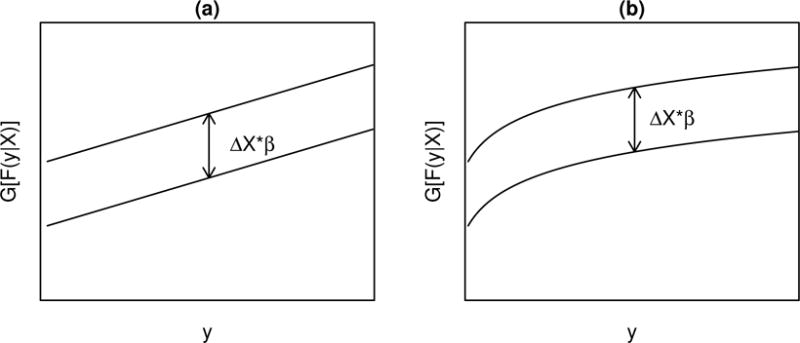
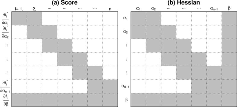
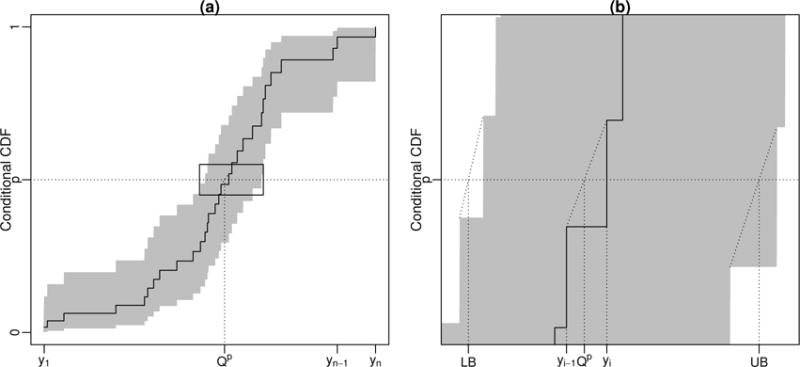
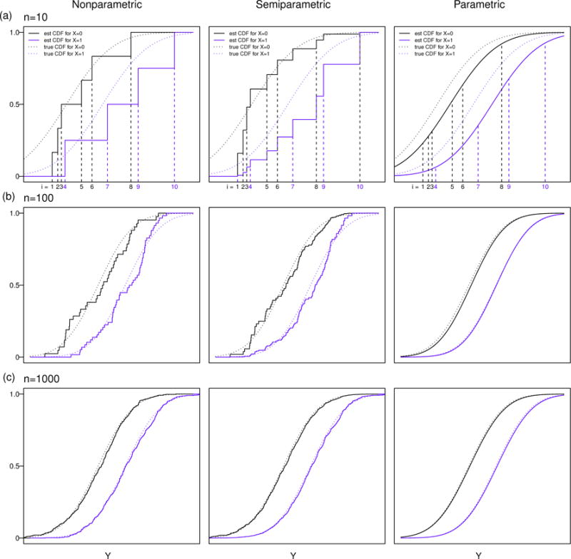
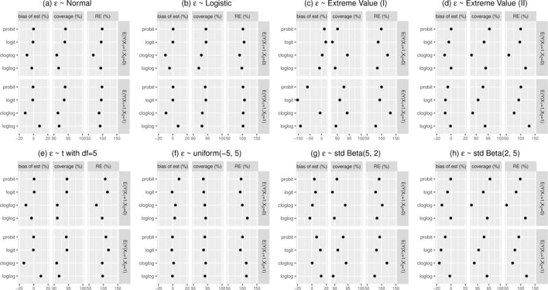
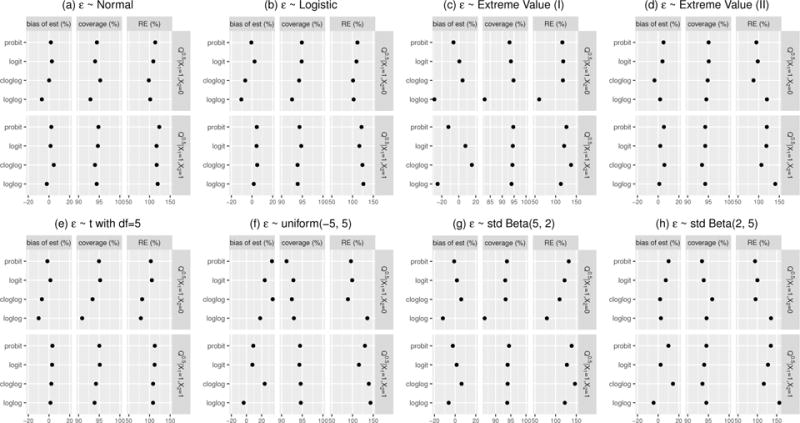
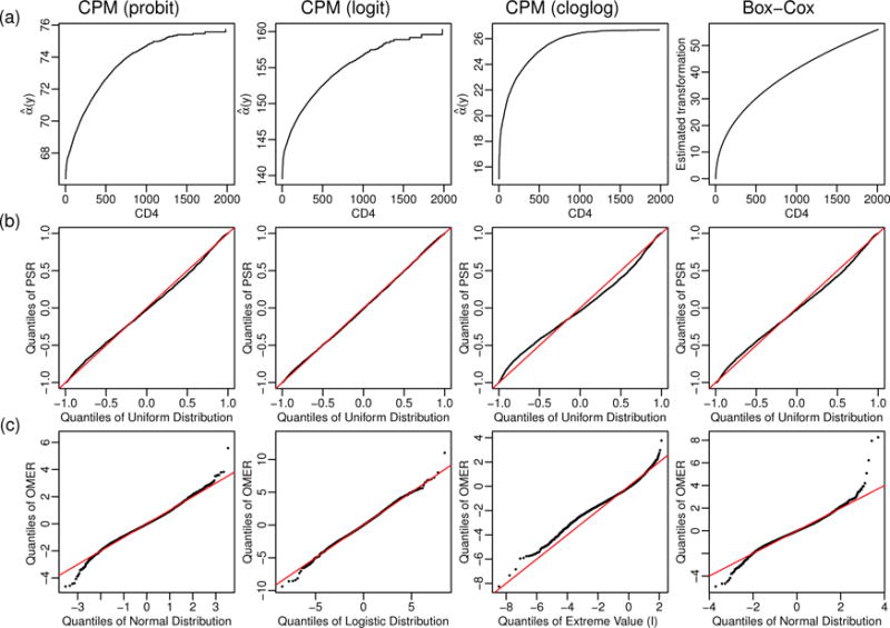
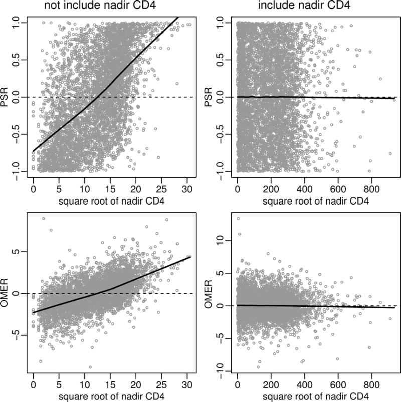
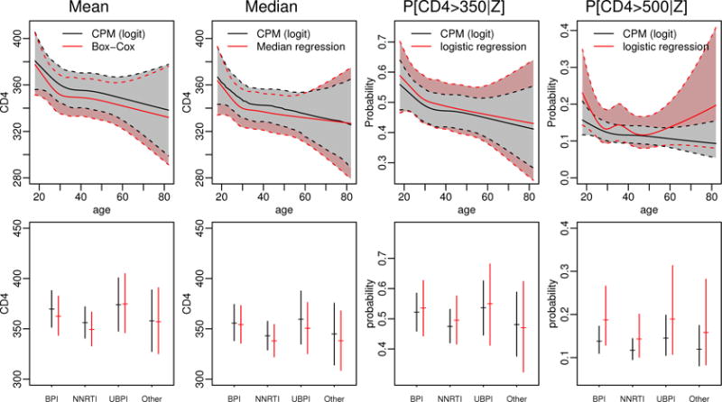
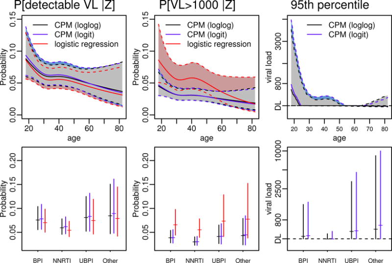
We study the application of a widely used ordinal regression model, the cumulative probability model (CPM), for continuous outcomes. Such models are attractive for the analysis of continuous response variables because they are invariant to any monotonic transformation of the outcome and because they directly model the cumulative distribution function from which summaries such as expectations and quantiles can easily be derived. Such models can also readily handle mixed type distributions. We describe the motivation, estimation, inference, model assumptions, and diagnostics. We demonstrate that CPMs applied to continuous outcomes are semiparametric transformation models. Extensive simulations are performed to investigate the finite sample performance of these models. We find that properly specified CPMs generally have good finite sample performance with moderate sample sizes, but that bias may occur when the sample size is small. Cumulative probability models are fairly robust to minor or moderate link function misspecification in our simulations. For certain purposes, the CPMs are more efficient than other models. We illustrate their application, with model diagnostics, in a study of the treatment of HIV. CD4 cell count and viral load 6 months after the initiation of antiretroviral therapy are modeled using CPMs; both variables typically require transformations, and viral load has a large proportion of measurements below a detection limit.

Keywords: nonparametric maximum likelihood estimation; ordinal regression model; rank-based statistics; semiparametric transformation model.

Figure 1

The parallelism assumptions in (a) the normal linear regression model Y = βX + ε with ε ~ N(0, 1) and (b) transformation models Y = H(βX + ε) with ε ~ F_ε, $G=F_{\epsilon }^{-1}$. Adapted from Harrell [2].

Figure 2

(a) Each observation’s contribution to the score function assuming observations are ordered by the value of y, i.e., y₁ < y₂ < ⋯ < y_n. White region indicates zero and grey region indicates non-zero values. (b) The bordered tridiagonal structure of Hessian matrix of log(L^∗) with respect to intercepts and slopes. Since α_i = α_j whenever y_i = y_j, the score function and Hessian matrix have similar forms when there are ties in the outcome.

Figure 3

(a): An estimated conditional CDF and its pointwise confidence intervals. (b): An illustration for estimating the p-th quantile of the conditional distribution, denoted as Q^p, and its confidence interval (LB, UB) through linear interpolation between y_i−1 and y_i, where $y_{\mathrm{i}}=\inf \left\{y:\widehat{F}\left(y|X\right)\ge p\right\}$, based on the estimated conditional CDF and its pointwise confidence intervals.

Figure 4

Estimation of conditional CDF from CPMs compared with parametric and nonparametric models in a simple example: (a) with a sample size of 10, (b) with a sample size of 100, and (c) with a sample size of 1000.

Figure 5

The performance of CPMs on estimating intercepts with n = 100: (i) ε ~ Normal and (ii) ε ~ Extreme Value (I).

Figure 6

The performance of CPMs on estimating the slopes β₁, β₂, and α(y) at y₁ = e⁻¹ ≈ 0.368, y₂ = e^−0.33 ≈ 0.719, y₃ = e^0.5 ≈ 1.649, y₄ = e^1.33 ≈ 3.781, and y₅ = e² ≈ 7.389 with properly specified link functions: (i) ε ~ Normal and (ii) ε ~ Extreme Value (I).

Figure 7

(i): The relative efficiency of properly specified CPM (using the probit link function) compared with properly specified Box-Cox transformation model; (ii): The relative efficiency of properly specified CPM (using the cloglog link function) compared with Cox proportional hazard model.

Figure 8

The performance of CPMs on estimating conditional CDF given X₁ = 1 and X₂ = 1, evaluated at y₁ = 0.368, y₂ = 0.719, y₃ = 1.649, y₄ = 3.781, and y₅ = 7.389 with properly specified link functions: (i) ε ~ Normal and (ii) ε ~ Extreme Value (I). The results are based on 10,000 simulation replicates for each sample size.

Figure 9

The performance of CPMs on estimating conditional means with commonly used link functions. We summarize the percent bias (%) of the point estimate, the coverage probability of 95% confidence intervals, and the relative efficiency (RE) for (X₁ = 1, X₂ = 0) and (X₁ = 1, X₂ = 1) with sample size of 100 in this plot. The percent bias of the point estimate is calculated as the mean of point estimates in 10,000 simulation replicates minus the true value and then divided by the true value. The RE is compared with properly specified linear regression measured with MSE ratio. Numerical summary of these results are provided in Supplemental Materials S.2.2.

Figure 10

The performance of CPMs on estimating medians with commonly used link functions. The description is similar as that for Figure 9 except that the RE is compared with properly specified median regression.

Figure 11

Average time to fit the cumulative probability model versus the average number of unique outcomes for different sample sizes, n. Results are based on 100 replications.

Figure 12

(a): the estimated intercepts â(y) from the CPMs using the probit, logit, and cloglog link functions, which can be interpreted as semiparametric estimates of the best transformation for the 6-month CD4 count. For purpose of comparison, we also plot the estimated Box-Cox transformation, (b): QQ-plots of probability-scale residuals (PSRs). (c): QQ-plots of observed-minus-expected residuals (OMERs), removing the residual for the observation with the largest value of 6-month CD4 count.

Figure 13

Residual-by-predictor plots using probability-scale residuals (PSRs) (top panel) and observed-minus-expected residuals (OMERs) on the transformed scale (bottom panel) from CPMs (using the logit link function) including and not including baseline nadir CD4 count in the models. Smoothed curves using Friedman’s super smoother are added.

Figure 14

The estimated mean, median, and the probabilities of CD4 being greater than 350 cells/μL and CD4 being greater than 500 cells/μL as functions of age (top panel) or treatment class (bottom panel, BPI: boosted protease inhibitors, NNRTI: non-nucleoside reverse transcriptase inhibitors, and UBPI: unboosted protease inhibitors) from the CPM with the logit link function fixing other predictors at their medians (for continuous variables) or modes (for categorical variables). For purpose of comparison, we also plot the conditional means from linear regression models with Box-Cox transformation, the conditional medians from median regression models, and conditional probabilities from logistic regression models using the dichotomized CD4 count as outcomes. The shaded regions are point-wise 95% confidence intervals.

Figure 15

The probabilities of 6-month viral load (VL) being detectable (≥ 400 copies/mL) and being greater than 1000 copies/mL, and the 95^th percentiles as functions of age (top panel) or treatment class (bottom panel), estimated using the CPM with the loglog and logit link functions, fixing other predictors at their medians (for continuous variables) or modes (for categorical variables). The shaded regions are the point-wise 95% confidence intervals. For purpose of comparison, we also show the estimates of the conditional probabilities from logistic regression models using the dichotomized viral load as the outcome. We also estimated conditional percentiles from quantile regression models by imputing the measurements below the detection limit to be the detection limit or 0. However, since the estimates from quantile regression models were very unstable with very wide 95% confidence intervals crossing 0, we did not plot the results.

References

1. Sall J. A monotone regression smoother based on ordinal cumulative logistic regression. ASA Proceedings of Statistical Computing Section. 1991:276–281.
1. Harrell FE. Regression Modeling Strategies: With Applications to Linear Models, Logistic and Ordinal Regression, and Survival Analysis. Second. Springer; 2015.
1. Walker SH, Duncan DB. Estimation of the probability of an event as a function of several independent variables. Biometrika. 1967;54(1–2):167–179. - PubMed
1. McCullagh P. Regression models for ordinal data. Journal of the Royal Statistical Society Series B (Methodological) 1980;42(2):109–142.
1. Fienberg SE. The Analysis of Cross-classified Categorical Data. Second. MIT Press; Cambridge, MA: 1980. (reprinted by Springer, New York, 2007)
Substances
LinkOut - more resources