High-Yield Methods for Accurate Two-Alternative Visual Psychophysics in Head-Fixed Mice

Abstract

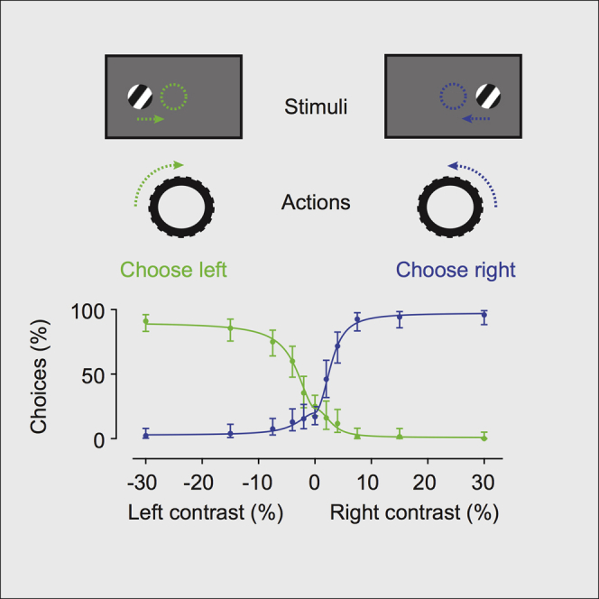
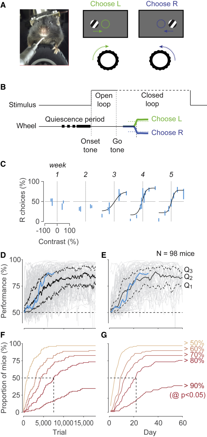
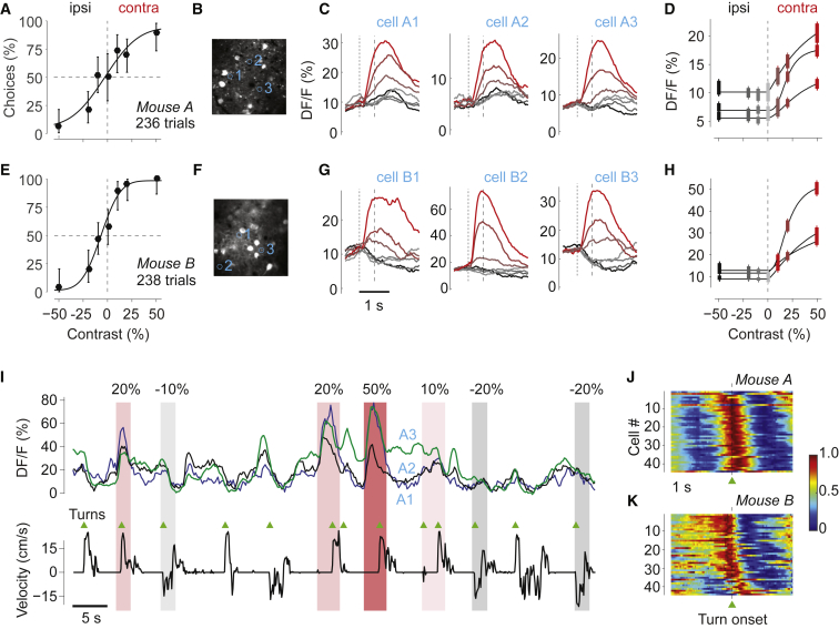
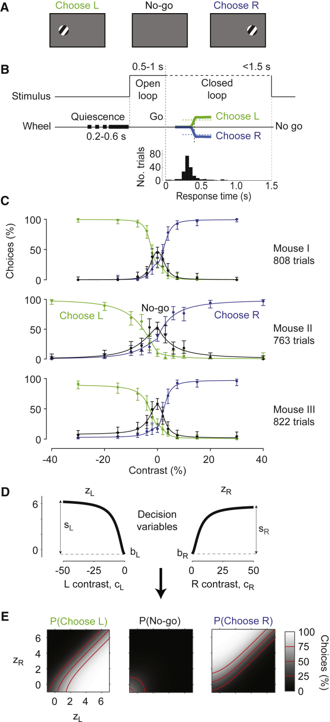
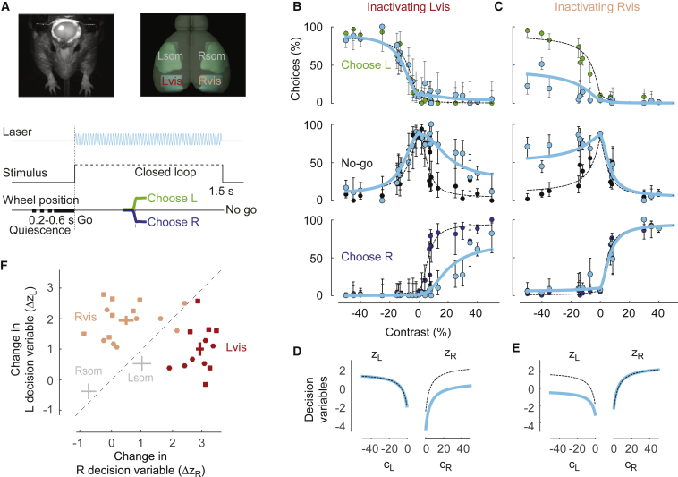
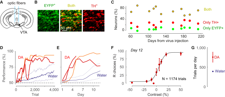
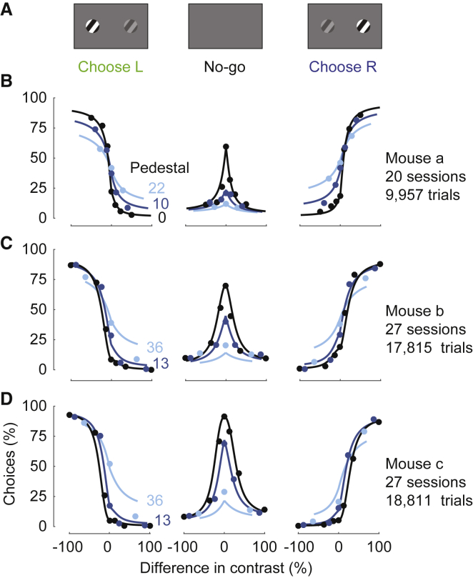
Research in neuroscience increasingly relies on the mouse, a mammalian species that affords unparalleled genetic tractability and brain atlases. Here, we introduce high-yield methods for probing mouse visual decisions. Mice are head-fixed, facilitating repeatable visual stimulation, eye tracking, and brain access. They turn a steering wheel to make two alternative choices, forced or unforced. Learning is rapid thanks to intuitive coupling of stimuli to wheel position. The mouse decisions deliver high-quality psychometric curves for detection and discrimination and conform to the predictions of a simple probabilistic observer model. The task is readily paired with two-photon imaging of cortical activity. Optogenetic inactivation reveals that the task requires mice to use their visual cortex. Mice are motivated to perform the task by fluid reward or optogenetic stimulation of dopamine neurons. This stimulation elicits a larger number of trials and faster learning. These methods provide a platform to accurately probe mouse vision and its neural basis.

Graphical abstract

Figure 1

The 2AFC Version of the Stimulus Detection Task (A) Left: a head-fixed mouse with forepaws on a steering wheel used to make choices. Right: at onset, the grating is either on the left or on the right, and the mouse turns the wheel (arrows) to move the grating to the center (dashed circles). (B) Time course of the basic task. Mice start the trial by holding the wheel still (quiescence). An onset tone may be played. The stimulus appears. Its position is initially fixed (open loop). After an optional go tone, stimuli become coupled with wheel position (closed loop). Choices are registered when the stimulus reaches the center of the screen (correct) or an equal distance in the opposite direction (incorrect). (C) Psychometric data obtained in the first 5 weeks for an example mouse. Bars show the percentage of times the mouse chose the right stimulus (95% binomial confidence intervals), as a function of stimulus contrast. By convention, we plot contrast of left stimuli as negative. Curves are fits with a psychometric curve. (D) Learning rates for a population of 98 mice. Performance is assessed on easy stimuli (≥40% contrast), as a function of number of trials. Blue trace highlights the example mouse in (C). Gray traces indicate performance by individual mice. Black traces indicate the 3 quartiles: the median (Q2) and the 25th and 75th percentiles (Q1 and Q3). The approximate chance level is 50% (dashed line). (E) Same as in (D), as a function of training days. (F) Cumulative probability of proportion of mice surpassing a given performance level as a function of trial number. (G) Same as in (F), as a function of training days. See also Figures S1–S3.

Figure 2

Imaging in V1 during the Task (A) Psychometric curve for an example mouse, measured during two-photon imaging in area V1. Error bars are 95% binomial confidence intervals. (B) Imaging field of view, with 3 cells circled and numbered. (C) Mean calcium activity averaged around the onset of the grating stimulus, grouped by stimulus condition (see color codes in next panel) for the 3 cells. Dotted line marks stimulus onset (preceded by a 2- to 3-s quiescence period). Dashed line marks the beginning of the closed-loop period, when the stimulus becomes movable. Data were taken from 181 trials (22–30 per condition). (D) Response amplitudes of each cell as a function of stimulus contrast. Positive and negative contrast denotes stimuli in the contralateral and ipsilateral visual fields. Amplitude is mean response at 1 s after grating onset. Curves indicates fits of the function $p+qf\left(c\right)$, with $f\left(c\right)$ defined in Equation 1. Error bars indicate SEM. (E–H) Same as (A)–(D), for a different mouse. Data were taken from 210 trials (24–43 per condition). (I) Example traces from the cells in (B)–(D) in the presence of stimuli of different contrasts (shaded areas) and in relation to wheel velocity (bottom trace). There are strong responses to the visual stimuli but also small responses synchronized with turn onsets (triangles). Onsets and offsets of wheel turns were identified by applying a dynamic threshold based on a Schmitt trigger to the wheel velocity traces. (J) Time course of movement-related activity in the absence of visual stimuli in 45 neurons from each of the 2 mice. Neurons were selected based on the quality of segmentation. We triggered calcium activity on wheel turn onsets, averaged across events, and normalized the results for each neuron (rows) to range from 0 to 1. Neurons were sorted by the amplitude 1 s before turn offset. (K) Same as in (J) for mouse B.

Figure 3

Elaboration of the Stimulus Detection Task in a 2AUC Version (A) In the 2AUC task, the mouse learns to choose left when the stimulus is on the left, choose right when the stimulus is on the right, and hold still (no-go) if the stimulus is absent. (B) Time course of the 2AUC task. At the go cue, the mouse has 1.5 s to move the wheel. Holding the wheel still for this period counts as a no-go choice. Histogram shows a typical distribution of response times in a session (time from go tone to response). (C) Choices as a function of stimulus contrast and position, for three sessions in 3 mice (rows). For each mouse, the data show the proportion of left (green), right (blue), and no-go choices (black) as a function of stimulus contrast. Negative contrast denotes stimuli appearing on the left side. Curves show fits of the probabilistic observer model. Error bars are 95% binomial confidence intervals. (D) The decision variables in the probabilistic observer model, with parameters obtained from mouse 1. The decision variables z_L and z_R grow with contrast presented on the left or on the right. Each function is defined by 2 parameters: bias, b, and sensitivity, s (Equations 1 and 2). (E) The probability of left, no-go, and right choices depends on the 2 decision variables. This dependence is parameter-free (Equation 3). See also Figure S4.

Figure 4

Effects of Optogenetic Inactivation of Visual Cortex (A) Methods of optogenetic inactivation during the 2AUC task. Top left: image of a mouse with the clear skull preparation, with laser spot on right hemisphere. Top right: illustration of the regions inactivated: left and right visual cortex (Lvis and Rvis) and, as a control, left and right somatosensory cortex (Lsom and Rsom). Inactivation of these regions was performed in different sessions. Bottom: time course of the task. In ∼33% of trials, stimuli were accompanied by laser illumination. (B) Effects of inactivation of left visual cortex. Proportion of left, no-go, and right choices as a function of stimulus contrast, under control conditions (green, black, and blue dots) and during optogenetic inactivation (cyan dots). Curves indicate fits of the probabilistic model under control conditions (dashed) and during optogenetic inactivation (cyan). Error bars show 95% binomial confidence intervals. Data were obtained in 6 sessions from 1 mouse. (C) Same as in (B), for inactivation of right visual cortex from the same mouse. Data were obtained in 7 sessions. (D) Decision variables obtained by the model fits in (B) as a function of contrast on the left and right in control condition (dashed) or during inactivation of left visual cortex (cyan). (E) Same as (D), for inactivation of right visual cortex. (F) Summary of the effects of optogenetic inactivation in the 4 regions outlined in (A). Effects are measured by the decrease in the left and right decision variables, $z_L$ or $z_R$, at 50% contrast. Dots indicate individual sessions from 2 mice (squares for the mouse in B–E, circles for another mouse) with inactivation of left visual cortex (red) or right visual cortex (pink). Crosses summarize the effects of inactivation in visual cortex (red and pink), and in somatosensory cortex (gray). The length of the crosses indicates ± SEM in the 2 dimensions. See also Figures S5 and S6.

Figure 5

Using Optogenetic Phasic Dopamine Stimulation to Train Mice in the Task (A) Schematic coronal section of the mouse brain (at the bregma, 3.1 mm) showing ventral tegmental area (VTA) and fiber optics implanted above VTA to elicit release of dopamine (DA). (B) Confocal images showing expression of ChR2-EYFP (green) in TH⁺ (DA) neurons (red) and overlay showing both (yellow). The bars quantify the specificity of expression, showing statistics of ChR2-EYFP and TH⁺ expression in midbrain neurons (n = 1,460 neurons counted in 121 confocal images acquired from 11 mice). (C) Stability of ChR2 expression in DAergic neurons (n = 11 mice). (D) Rapid learning of the task in 3 mice receiving DA stimulation as a reward. Red and orange lines show rapid increase in the performance of naive mice that were solely trained with optogenetic DA stimulation. Blue curves show results for mice that trained with water reward (median and quartile ranges, replotted from Figure 1). (E) Same as in (D), as a function of training day. (F) Psychometric function obtained from example animal (orange line in C and D) on the 12^th day of behavioral training. Error bars show 95% binomial confidence intervals. (G) Mean trials per day of mice receiving DA stimulation (red) compared to water reward (blue). Error bars represent SEM (smaller than the dot for water reward).

Figure 6

Extension of the 2AUC Task to the Study of Contrast Discrimination (A) Stimulus conditions used in the discrimination task. Gratings are presented on both sides and the mouse is rewarded for choosing the side with the highest contrast, or opting for no-go if both contrasts are zero. (B) Psychometric data from 1 mouse. Panels show left choices, no-go choices, and right choices, as a function of the difference between left and right contrast (c_R-c_L). Colors indicate the pedestal contrast, i.e., the minimum contrast present on the screen, min(c_L,c_R). (C and D) Same as in (B) for 2 more mice.

References

1. Abrahamyan A., Silva L.L., Dakin S.C., Carandini M., Gardner J.L. Adaptable history biases in human perceptual decisions. Proc. Natl. Acad. Sci. USA. 2016;113:E3548–E3557. - PMC - PubMed
1. Albrecht D.G., Hamilton D.B. Striate cortex of monkey and cat: contrast response function. J. Neurophysiol. 1982;48:217–237. - PubMed
1. Andermann M.L., Kerlin A.M., Reid R.C. Chronic cellular imaging of mouse visual cortex during operant behavior and passive viewing. Front. Cell. Neurosci. 2010;4:3. - PMC - PubMed
1. Bak J.H., Choi J.Y., Akrami A., Witten I.B., Pillow J. Adaptive optimal training of animal behavior. In: Lee D.D., Sugiyama M., Luxburg U.V., Guyon I., Garnett R., editors. Advances in Neural Information Processing Systems. MIT Press; 2016. pp. 1947–1955.
1. Beck J.A., Lloyd S., Hafezparast M., Lennon-Pierce M., Eppig J.T., Festing M.F., Fisher E.M. Genealogies of mouse inbred strains. Nat. Genet. 2000;24:23–25. - PubMed
LinkOut - more resources