Standardized mean differences cause funnel plot distortion in publication bias assessments

Abstract

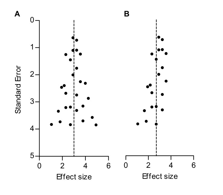
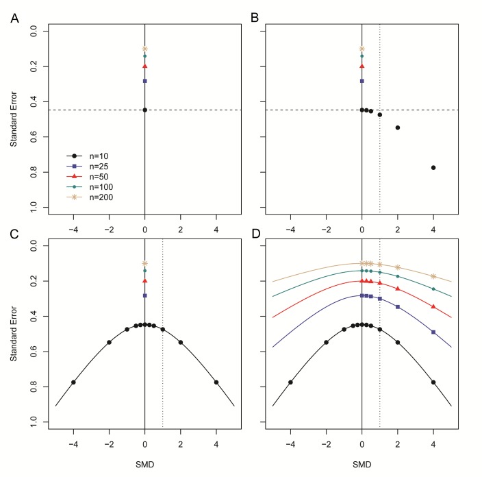
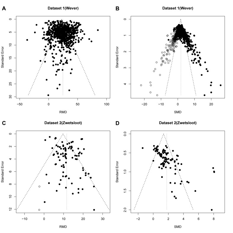
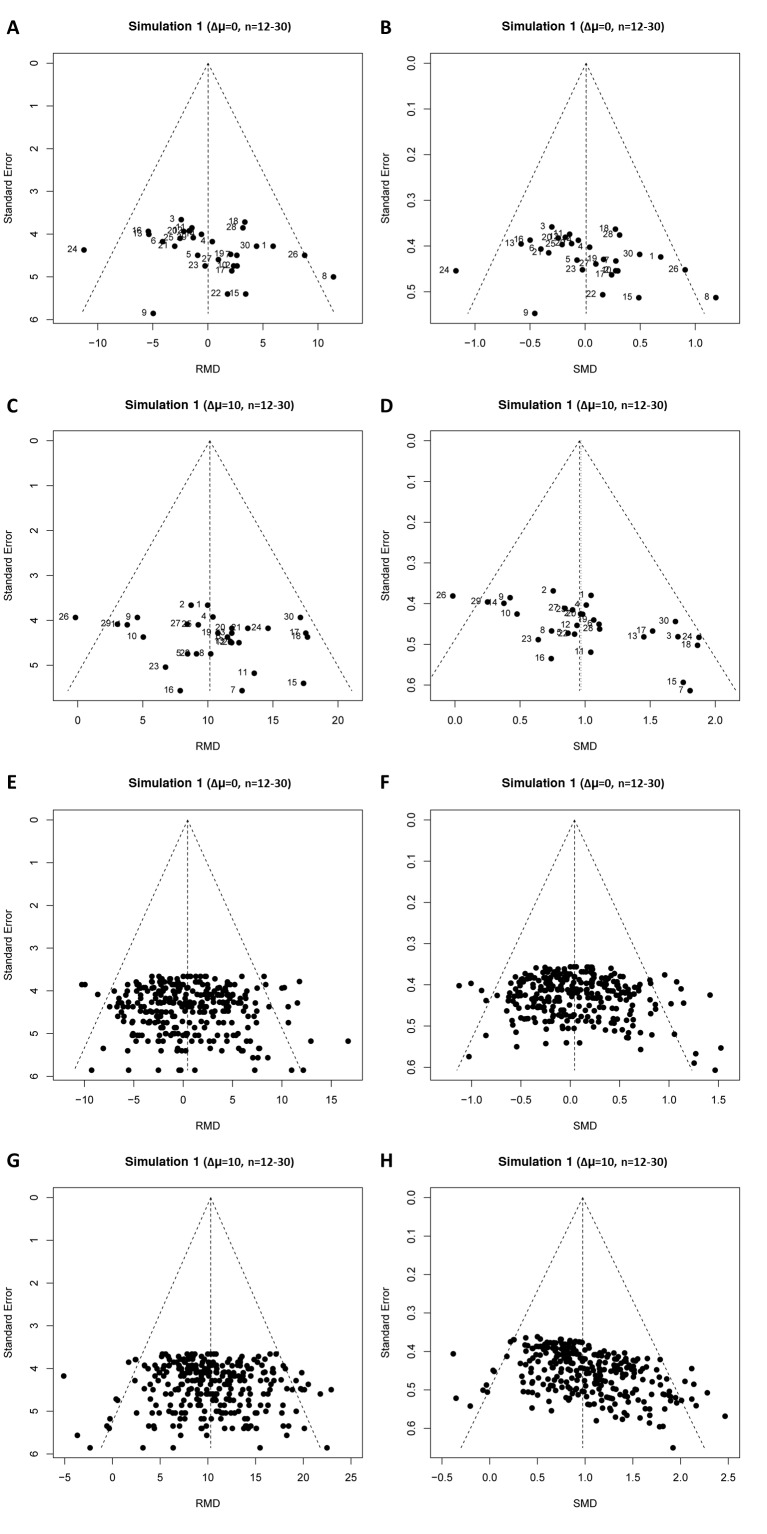
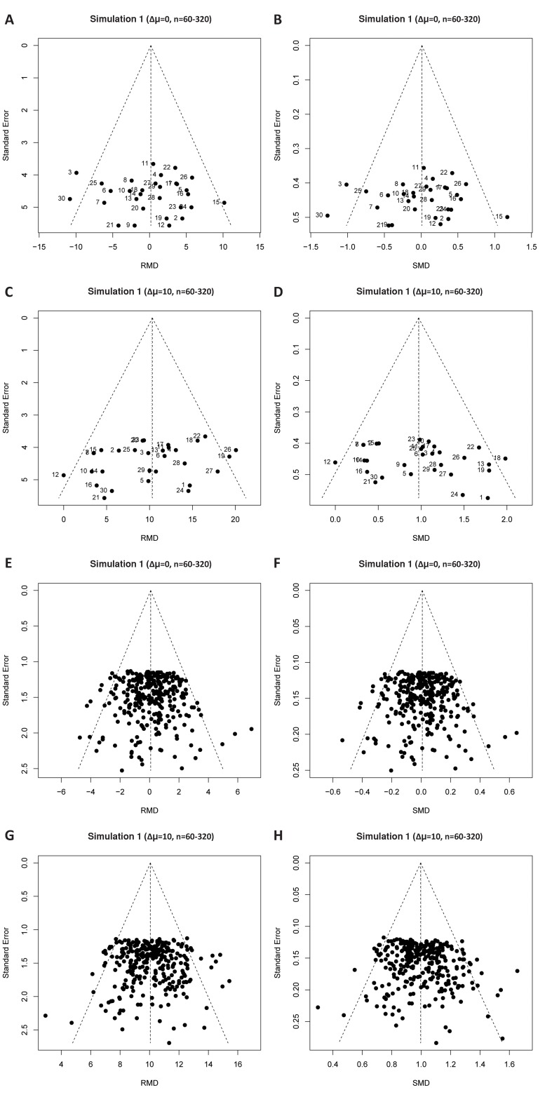
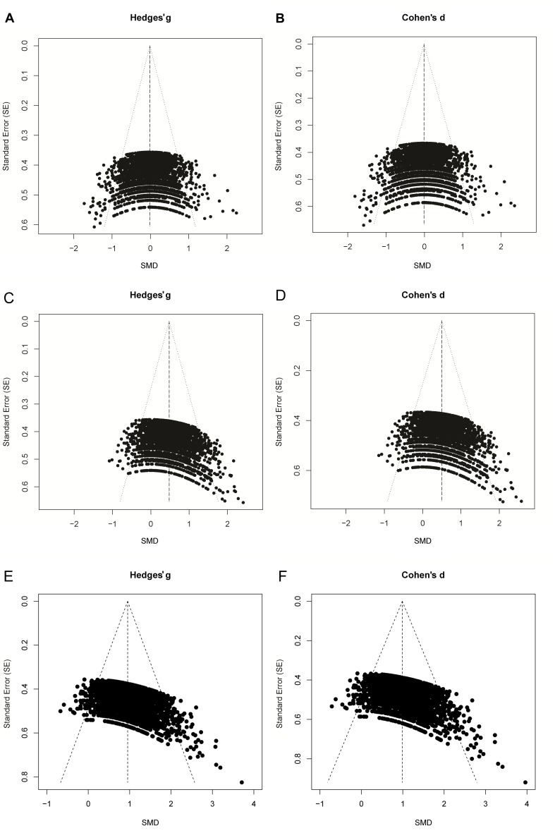
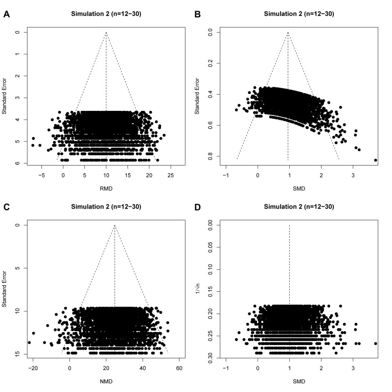
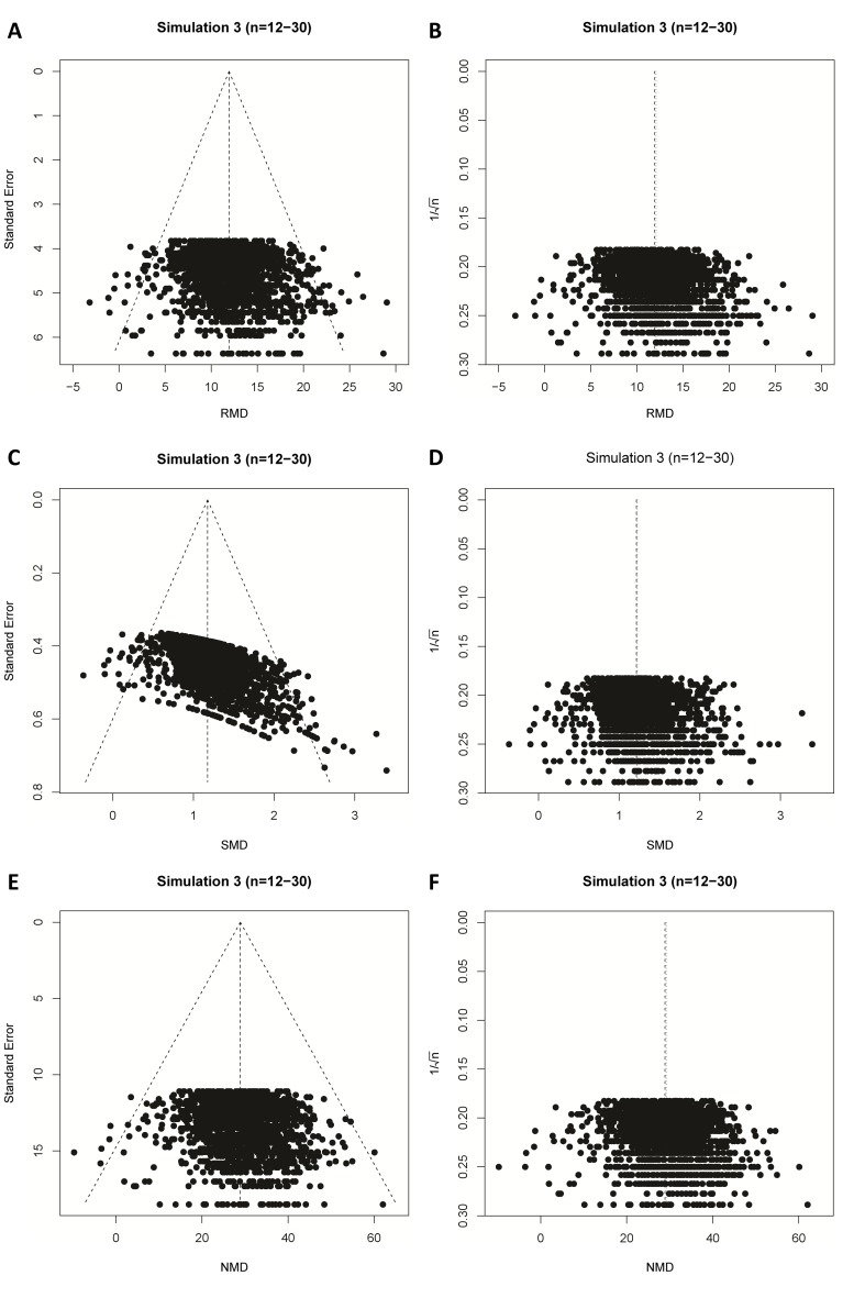
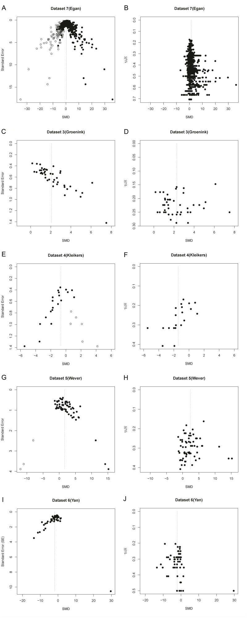
Meta-analyses are increasingly used for synthesis of evidence from biomedical research, and often include an assessment of publication bias based on visual or analytical detection of asymmetry in funnel plots. We studied the influence of different normalisation approaches, sample size and intervention effects on funnel plot asymmetry, using empirical datasets and illustrative simulations. We found that funnel plots of the Standardized Mean Difference (SMD) plotted against the standard error (SE) are susceptible to distortion, leading to overestimation of the existence and extent of publication bias. Distortion was more severe when the primary studies had a small sample size and when an intervention effect was present. We show that using the Normalised Mean Difference measure as effect size (when possible), or plotting the SMD against a sample size-based precision estimate, are more reliable alternatives. We conclude that funnel plots using the SMD in combination with the SE are unsuitable for publication bias assessments and can lead to false-positive results.

Keywords: data simulation; epidemiology; funnel plot; global health; human biology; medicine; meta-analysis; none; publication bias.

Figure 1.. Hypothetical funnel plots in the absence (A) and presence (B) of bias.

The precision estimate used is the standard error (SE). Dashed lines indicate the summary effect estimate.

Figure 2.. Step-wise illustration of distortion in SMD versus SE funnel plots.

(A) Depicted are simulated studies with a sample size of respectively 10 (large black circles), 25 (blue squares), 50 (red triangles), 100 (small green circles) and 200 (gold asterisks) subjects per group, and an SMD of zero. The SE of these studies (indicated by the dashed line for studies with n = 10) solely depends on their sample size, as SMD² = 0 and therefore does not contribute to the equation for the SE. As expected, the SE decreases as the sample size increases. (B) Five data points from simulated studies with n = 10 and a stepwise increasing SMD are added to the plot. For these studies, the SMD² contributes to the equation for the SE, and the SE will decrease even though the sample size is constant. The dotted line represents a hypothetical summary effect of SMD = 1 in a meta-analysis. Note that when assessing a funnel plot for asymmetry around this axis, the data points with an SMD < 1 have skewed to the upper left-hand region, whereas studies with an SMD > 1 are in the lower right region of the plot. This distortion worsens as the SMD increases. (C) Because the SMD is squared in the equation for the SE, the same distortion pattern is observed for negative SMDs. Thus, funnel plots will be distorted most when the study samples sizes are small and SMDs are either very positive or very negative. (D) The same deviation is observed for simulated studies with larger sample sizes, however, the deviation decreases as the sample size increases, because the sample size will outweigh the effect of SMD² in the equation for the SE.

Figure 3.. Reanalysis of data from Wever et al.

(A,B) and Zwetsloot et al. (C,D), with funnel plots based on raw mean difference (RMD; A,D) or standardized mean difference (SMD; B,D). Filled circles = observed data points; open circles = missing data points as suggested by trim and fill analysis.

Figure 4.. Representative raw mean difference (RMD; A, C, E, G) and standardized mean difference (Hedges’ g SMD; B, D, F, H) funnel plots for simulated unbiased meta-analyses containing thirty (A–D) or 300 (E–H) studies with a small sample size (total study n = 12–30).

Simulations were performed without an intervention effect (Δμ = 0; A–B and E–F), or with an intervention effect (Δμ = 10; C–D and G–H). Δμ = difference in normally distributed means between control and intervention group. Representative funnel plots for studies with a large sample size (total study n = 60–320) are shown in Figure 4—figure supplement 1. Representative funnel plots for the comparison between Hedges’ g and Cohen’s d are shown in Figure 4—figure supplement 2.

Figure 4—figure supplement 1.. Simulation 1 funnel plots for large study sample sizes.

Figure 4—figure supplement 2.. Funnel plots comparing Cohen’s d versus Hedges g.

Figure 5.. raw mean difference (RMD; A), standardized mean difference (SMD; B), normalized mean difference (NMD; C) with SE as precision estimate, and SMD funnel plots using 1/√n as precision estimate (D).

All plots show the same simulated meta-analysis containing 3000 studies with small sample sizes (n = 12–30) and an overall intervention effect of Δμ = 10. Δμ = difference in normally distributed means between control and intervention group.

Figure 6.. Simulation 3 funnel plots of biased meta-analyses.

Representative funnel plots of simulated biased meta-analyses using a raw mean difference (RMD; A–B), a standardized mean difference (SMD; C–D), or a normalised mean difference (NMD; E–F) effect measure. The present example contains 3000 studies with a small study sample size (n = 12–30) and an intervention effect present (difference in normal distribution means between control and intervention group = 10). Publication bias was introduced stepwise, by removing 10% of primary studies in which the difference between the intervention and control group means was significant at p<0.05, 50% of studies where the significance level was p≥0.05 to p<0.10, and 90% of studies where the significance level was p≥0.10. Precision estimates are standard error (A, C, E) or sample size-based (B, D, F), where n = total primary study sample size.

Figure 7.. Funnel plots of re-analysis of empirical meta-analyses.

Funnel plots of empirical meta-analyses plotted as standardized mean difference (SMD) versus standard error, as in the original publications (left hand panels), and as SMD versus 1/√n after re-analysis. n = total primary study sample size; filled circles = observed data points; open circles = missing data points as suggested by trim and fill analysis.

References

1. Bastian H, Glasziou P, Chalmers I. Seventy-five trials and eleven systematic reviews a day: how will we ever keep up? PLoS Medicine. 2010;7:e1000326. doi: 10.1371/journal.pmed.1000326. - DOI - PMC - PubMed
1. Begg CB, Mazumdar M. Operating characteristics of a rank correlation test for publication bias. Biometrics. 1994;50:1088–1101. doi: 10.2307/2533446. - DOI - PubMed
1. Chalmers I, Bracken MB, Djulbegovic B, Garattini S, Grant J, Gülmezoglu AM, Howells DW, Ioannidis JP, Oliver S. How to increase value and reduce waste when research priorities are set. The Lancet. 2014;383:156–165. doi: 10.1016/S0140-6736(13)62229-1. - DOI - PubMed
1. Cohen J. Statistical Power Analysis for the Behavioral Sciences. 2nd ed. Hillsdale: Lawrence Erlbaum; 1988.
1. Dragulescu AA. xlsx: Read, write, format Excel 2007 and Excel 97/2000/XP/2003 files. 0.5.7R Package. 2014 https://CRAN.R-project.org/package=xlsx
Publication types