Dynamic Neural Fields with Intrinsic Plasticity

Abstract

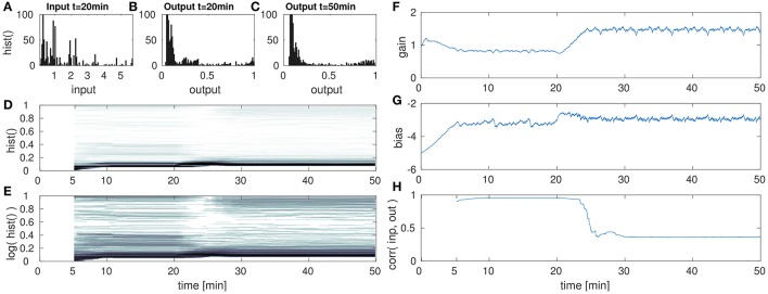
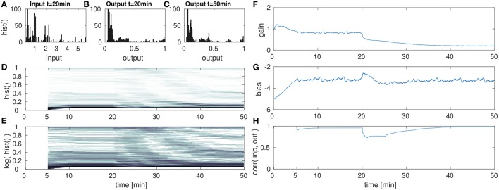
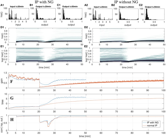
Dynamic neural fields (DNFs) are dynamical systems models that approximate the activity of large, homogeneous, and recurrently connected neural networks based on a mean field approach. Within dynamic field theory, the DNFs have been used as building blocks in architectures to model sensorimotor embedding of cognitive processes. Typically, the parameters of a DNF in an architecture are manually tuned in order to achieve a specific dynamic behavior (e.g., decision making, selection, or working memory) for a given input pattern. This manual parameters search requires expert knowledge and time to find and verify a suited set of parameters. The DNF parametrization may be particular challenging if the input distribution is not known in advance, e.g., when processing sensory information. In this paper, we propose the autonomous adaptation of the DNF resting level and gain by a learning mechanism of intrinsic plasticity (IP). To enable this adaptation, an input and output measure for the DNF are introduced, together with a hyper parameter to define the desired output distribution. The online adaptation by IP gives the possibility to pre-define the DNF output statistics without knowledge of the input distribution and thus, also to compensate for changes in it. The capabilities and limitations of this approach are evaluated in a number of experiments.

Keywords: adaptation; dynamic neural fields; dynamics; intrinsic plasticity.

Figure 1

Illustration of three different distributions of a “circularity feature” obtained from sensory input. On the vertical axis, the circularity is denoted, which determines the activation level of a DNF; the horizontal axis shows the probability to measure the respective circularity value. The green filling represents a fixed fraction (20%) of the total probability density.

Figure 2

The three regimes of stability. (Left column): Phase plots for different regimes of the DNF equation for a zero-dimensional feature space x (u is a scalar value). Black dots indicate stable fixed points, empty circles—unstable fixed points. (Right column): The output g(u) of a DNF is illustrated (in red) for an one-dimensional feature space x. The blue-dashed line represents the input S(x). The arrows depict qualitative changes in the regimes of stability determined by the input strength S(x).

Figure 3

Sketch of the gain adaptation in Equation (10) (right) and the bias adaptation in Equation (16) (left) for μ = 0.2, input z(t) in the range of [0, 1], a learning rate η = 1, and a current gain of 1.

Figure 4

Sketch of the input encoding used for evaluation of DNFs with IP, illustrated for two tactile contacts at opposing orientations (x = 95 deg and x = 275 deg). A population of neurons encode the contact circularity over contact orientation, with each neuron encoding a specific orientation. The corresponding neurons representing the orientations of the tactile inputs are activated and their response strength is related to the contact circularity of the tactile contacts (the two black bars). The Gaussian blurring of the neuronal activation to neighboring neurons (encoding similar orientations) is depicted in the blue bars. This population representation of tactile inputs is done for every time step, leading to the input time series S(x, t).

Figure 5

Selection of the input time sequence S(x, t) and the corresponding DNF output g(u(x, t)) for converged gain and bias adaptation. Time is on the horizontal axis and the one dimensional population code is on the vertical axis. (Top) The input time series S(x) to the DNF. Here, the gray level encodes the input amplitude S(x) at the corresponding contact orientation x (vertical axis) for a point in time. (Middle) (μ = 0.1): the DNF output for the converged IP parameters (a = 0.65 and b = −3.5). The input-output correlation (Equation 17) for the shown sequence is 0.69. (Bottom) The DNF output for the converged IP parameters (a = 0.59 and b = −3.0) for μ = 0.2. The input-output correlation is 0.67. In the middle and bottom plots, the gray level encodes the DNF output activity g(u), i.e., surface detection at the corresponding contact orientation x (vertical axis).

Figure 6

DNF with IP for low amplitude input after the 20th min. (A) DNF input histogram, z(t), (B) DNF output histogram, y(t) after IP parameter convergence at the 20th min. (C) DNF output histogram, y(t) at the 50th min after the input down-scaling. (D) DNF output histogram over time, (E) logarithmic version of (D), (F–H) gain, bias and the input-output correlation over time, respectively. See text for further description.

Figure 7

DNF with IP for high amplitude input after the 20th min. (A) DNF input histogram z(t), (B) DNF output histogram, y(t), after IP parameter convergence at the 20th min. (C) DNF output histogram at the 50th min after the input up-scaling. (D) DNF output histogram over time, (E) logarithmic version of (D), (F–H) gain, bias and the input-output correlation over time, respectively. See text for further description.

Figure 8

DNF with IP and shifted input after the 20th min with- and without the natural gradient. On the left three top rows show the results for IP with natural gradient descent. The right three rows show the results when using the gradient descent in euclidean parameter space. Shown are the input z(t) (A) and output y(t) (B,C) histograms of the DNF. The output histograms over time (D,E) show the output distributions over time, computed by a sliding time window of 5 min. See text for further description. The lowest three rows show parameter adaptation in a DNF with IP and shifted input after the 20th min with- and without the natural gradient. The parameter adaptation is shown for the gain (F) and bias (G), and the input-output correlation (H) is plotted. The experiment with NG is stopped after the 50th min, the experiment without NG is run until minute 100. See text for further description.

References

1. Amari S. (1977). Dynamics of pattern formation in lateral-inhibition type neural fields. Biol. Cybern. 27, 77–87. - PubMed
1. Amari S. (1998). Natural gradient works efficiently in learning. Neural Comput. 10, 251–276.
1. Barth A. L., Poulet J. F. (2012). Experimental evidence for sparse firing in the neocortex. Trends Neurosci. 35, 345–355. 10.1016/j.tins.2012.03.008 - DOI - PubMed
1. Bicho E., Erlhagen W., Louro L., Costa e Silva E. (2011). Neuro-cognitive mechanisms of decision making in joint action: a human-robot interaction study. Hum. Mov. Sci. 30, 846–868. 10.1016/j.humov.2010.08.012 - DOI - PubMed
1. Boedecker J., Obst O., Mayer N., Asada M. (2009a). Initialization and self-organized optimization of recurrent neural network connectivity. HFSP J. 3, 340–349. 10.2976/1.3240502 - DOI - PMC - PubMed