

Principal components analysis in clinical studies
- PMID: 28936445
- PMCID: PMC5599285
- DOI: 10.21037/atm.2017.07.12
Principal components analysis in clinical studies
Abstract
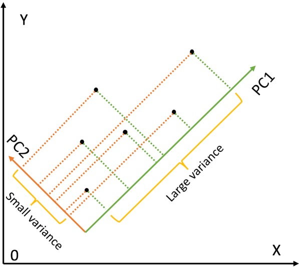
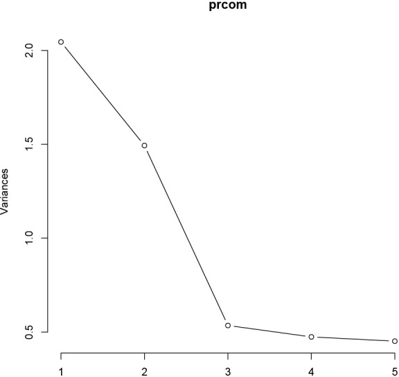
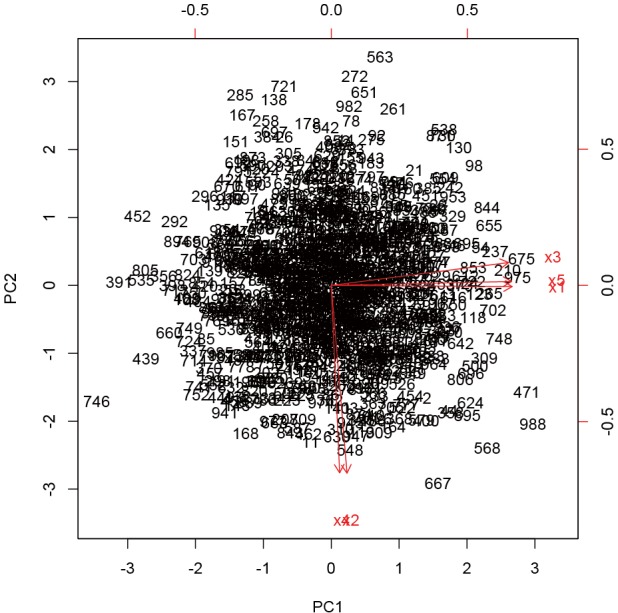
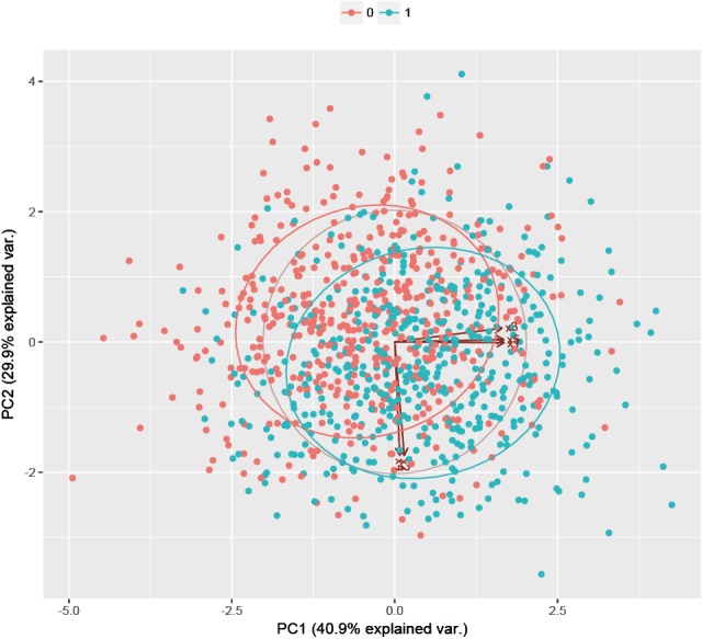
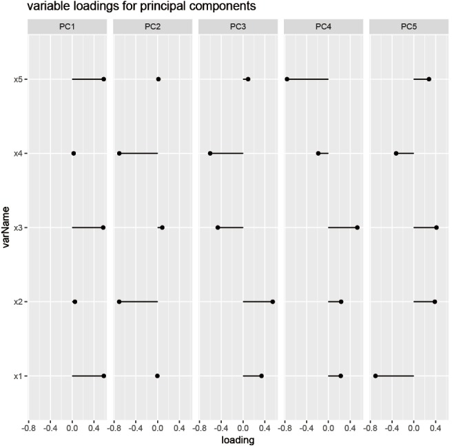
In multivariate analysis, independent variables are usually correlated to each other which can introduce multicollinearity in the regression models. One approach to solve this problem is to apply principal components analysis (PCA) over these variables. This method uses orthogonal transformation to represent sets of potentially correlated variables with principal components (PC) that are linearly uncorrelated. PCs are ordered so that the first PC has the largest possible variance and only some components are selected to represent the correlated variables. As a result, the dimension of the variable space is reduced. This tutorial illustrates how to perform PCA in R environment, the example is a simulated dataset in which two PCs are responsible for the majority of the variance in the data. Furthermore, the visualization of PCA is highlighted.
Keywords: Principal component analysis; R; multicollinearity; regression.
Conflict of interest statement
Conflicts of Interest: The authors have no conflicts of interest to declare.
Figures
References
-
- Burt C. Factor analysis and canonical correlations. Br J Psychol 1948;1:95-106.
-
- Rencher AC. editor. Principal Component Analysis. 2nd ed. New York: John Wiley & Sons, Inc, 2002.
Publication types
LinkOut - more resources
Full Text Sources
Other Literature Sources
Research Materials