Two-photon calcium imaging of the medial prefrontal cortex and hippocampus without cortical invasion

Abstract

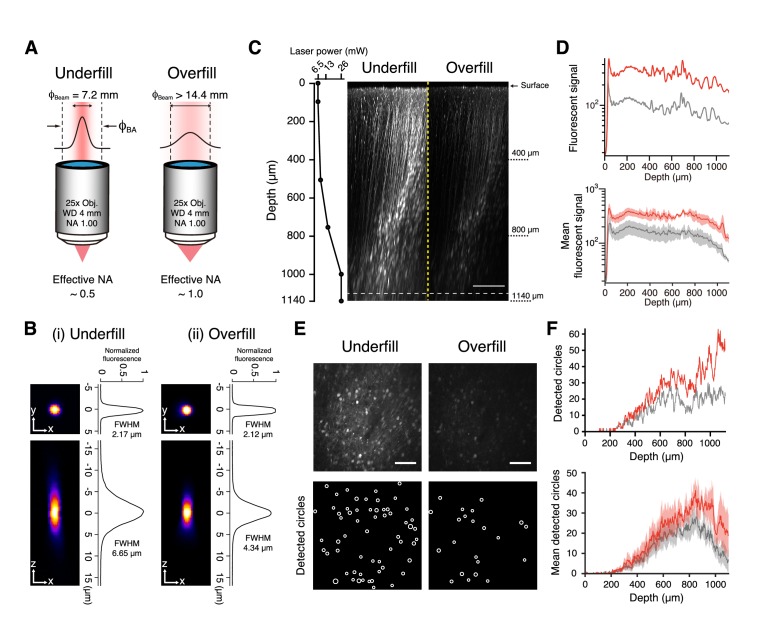
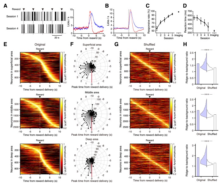
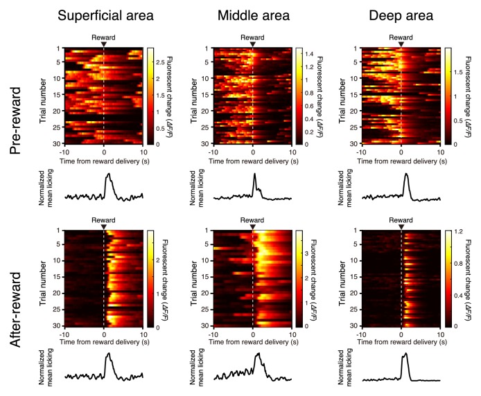
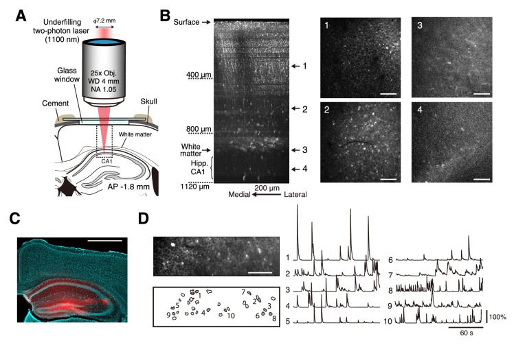
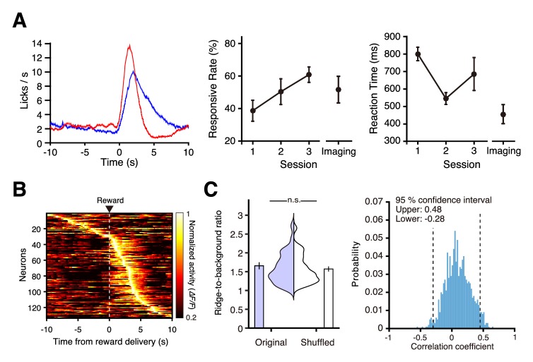
In vivo two-photon calcium imaging currently allows us to observe the activity of multiple neurons up to ~900 µm below the cortical surface without cortical invasion. However, many important brain areas are located deeper than this. Here, we used an 1100 nm laser that underfilled the back aperture of the objective together with red genetically encoded calcium indicators to establish two-photon calcium imaging of the intact mouse brain and detect neural activity up to 1200 μm from the cortical surface. This imaging was obtained from the medial prefrontal cortex (the prelimbic area) and the hippocampal CA1 region. We found that neural activity before water delivery repeated at a constant interval was higher in the prelimbic area than in layer 2/3 of the secondary motor area. Reducing the invasiveness of imaging is an important strategy to reveal the intact brain processes active in cognition and memory.

Keywords: Hippocampus; Prefrontal cortex; Two-photon imaging; mouse; neuroscience.

Figure 1.. Two-photon imaging with underfilled and overfilled objectives.

(A) Schematic illustration of an objective with NA of 1.0, magnification of 25, and working distance of 4 mm, which was underfilled (left) and overfilled (right) with an excitation laser. ‘Underfill’ and ‘Overfill’ denote that 1/e²-width of the excitation laser beam,ϕ_Beam, is narrower and wider than the back aperture of the objective, ϕ_BA, respectively. The calculated effective NAs are indicated below. (B i, ii) Representative XY (left top) and XZ (left bottom) images of a 2 µm fluorescence bead and their profile (right) when the objective was underfilled (i) and overfilled (ii). (C) Representative XZ images of mFrC expressing tdTomato in the underfilled and overfilled configurations (right images). The laser power was determined at six depth points (dots) and gradually increased between dots as the depth increased (left graph). The power at each cortical depth was equal in both underfilled and overfilled configurations. Contrast was not enhanced in either image. The images are the maximum intensity projection of XYZ images along the Y axis. Scale bar, 200 µm. (D) Top, Z profiles of the mean fluorescence signals from the brightest pixels from the same volume as in (C) in the underfilled (red) and overfilled (gray) configurations. Bottom, Z profiles of fluorescence signals averaged over four volumes from two mice. Light shading indicates the s.e.m. (E) XY images in the underfilled (left) and overfilled (right) configurations at the depth indicated by the dotted line in (C), 1060 µm from the brain surface. Contrast enhancement was not performed in these images. Bottom, spatial distributions of circles detected by the Hough transform method. Scale bar, 100 µm. (F) Top, Z profiles of the number of detected circles from the same volume as in (C) in the underfilled (red) and overfilled (gray) configurations. Bottom, Z profiles of the number of detected circles averaged over four volumes from two mice. Light shading indicates the s.e.m.

Figure 2.. Two-photon calcium imaging of intact medial frontal cortex.

(A) Schematic illustration of in vivo two-photon imaging of the mFrC. The dotted square indicates the location at which the Z-stack images in (B) were acquired. Imaging stage was tilted so that the glass window was perpendicular to the optical axis (see Materials and methods). FrC, frontal cortex; PL, prelimbic area. Immersion water was placed between the objective and the cranial window, but is not illustrated for visual clarity. (B) Left, representative XZ image of mFrC expressing R-CaMP1.07. The images are maximum intensity projections of XYZ images along the Y axis. These were acquired in awake mice, and the multiple horizontal dark lines are motion artifacts. Scale bar, 200 µm. Middle and right, four XY images at the depths indicated by the number at the left. Scale bar, 100 µm. (C) Expression of R-CaMP1.07 (red) and cell nuclei (NeuroTrace 435, cyan) after imaging 11 fields at depths of 340–1140 µm for 5 days. The total duration of imaging was 200 min. Scale bar, 1 mm. (D) Left, representative time-averaged XY image of mFrC expressing R-CaMP1.07 at a depth of 1030 µm. Scale bar, 100 µm. Right, spatial distribution of neurons identified by the constrained non-negative matrix factorization (cNMF) algorithm. (E) Calcium transient traces for the numbered filled contours are shown in (D). These measurements were taken while the animal was quiet, more than 15 min after the conditioning experiment.

Figure 3.. Immunoreactivity after deep imaging of the medial frontal cortex.

(A–C) Top, representative expression of GFAP (A), Iba1 (B), and HSP70/72 (C) in contralateral (left) and imaged (right) hemispheres. Scale bar, 500 µm. Middle and bottom, expanded images of the numbered boxes, including the cortical surface (middle) and imaging sites (bottom). Scale bar, 100 µm. (D–F) Ratios of expression intensity for GFAP (D), Iba1 (E), and HSP70/72 (F) in the AAV-injected hemisphere compared with the contralateral hemisphere. Each dot indicates the ratio in each slice that included both hemispheres. Without imaging: mice with only AAV injections and cranial windows (10 slices from two mice as a negative control for GFAP and Iba1; four slices from one mouse as a negative control for HSP70/72). 15 min and 30 min deep: after 15-min imaging at 800–900 µm depths (eight slices from two mice for GFAP; 10 slices from two mice for Iba1; 15 slices from two mice for HSP70/72) and after 30-min imaging at 900–1100 µm depths (21 slices from four mice for GFAP; 21 slices from four mice for Iba1; 12 slices from two mice for HSP70/72), respectively; 30 min shallow: after 30 min imaging at 300–400 µm depths (eight slices from two mice for GFAP; 10 slices from two mice for Iba1; 10 slices from two mice for HSP70/72); 30 min shallow at 920 nm: after 30-min imaging at 200–300 µm depths (overfilled with 200 mW, 920 nm laser in the slow scanning mode) (seven slices from two mice for GFAP; six slices from two mice for Iba1; six slices from two mice for HSP70/72). Shaded areas indicate the mean ±2 s.d. of the immunoreactivity in the negative control experiment. Horizontal bars indicate significant differences (**: p<0.01,***: p<0.001, one-way ANOVA with Tukey-Kramer method for post-hoc multiple comparisons, see Figure 3—source data 1). Pairs without bar were not significantly different (see Figure 3—source data 1).

Figure 3—figure supplement 1.. Immunoreactivity in the negative control experiment.

(A–C) Top, representative expression of GFAP (A), Iba1 (B), and HSP70/72 (c) in contra lateral (left) and AAV-injected and cranial window-set (right) hemispheres. Scale bar, 200 µm. Middle and bottom, expanded images corresponding to the numbered boxes, including the cortical surface (middle) and imaging sites (bottom). Scale bar, 100 µm.

Figure 3—figure supplement 2.. Immunoreactivity in the strong positive control experiment.

(A–C) Representative expressions of GFAP (A), Iba1 (B), and HSP70/72 (C) in contralateral (left) and imaged (right) hemispheres (30 min imaging at 300 µm depth was conducted with a 200 mW, 920 nm laser with an overfilled objective in the slow scanning mode). Scale bar, 200 µm.

Figure 3—figure supplement 3.. Calcium transients of neurons in the deep area before and after 15 min imaging.

(A) Representative calcium-transient traces from neurons at a depth of 1040 µm during the first 5-min period and the last 5-min period of the total 25-min imaging. The same number indicates the same neuron. (B) Mean inferred activities during the first 5 min and last 5 min of the total 25-min imaging. For each neuron, the activity was inferred from the fluorescent signal with spike deconvolution in the cNMF algorithm. The difference was not significant (p=0.22, n = 63 neurons from 2 mice, paired t-test).

Figure 4.. Neural activity in the medial frontal cortex during conditioning.

(A) Left, representative traces of licking behavior during conditioning sessions 1 (top) and 4 (bottom) from the same mouse. Lines indicate the timing of licking detected by cut-off of light to an infrared LED sensor. Dashed vertical lines indicate the timing of water delivery. Right, mean licking frequency aligned with water delivery for sessions 1 (red) and 4 (blue) from the same mouse as in the left panel. Light shading indicates the s.e.m. (B) Mean licking frequency for sessions 1 (red) and 4 (blue; n = 11 mice). Light shading indicates the s.e.m. (C) Response rate in conditioning sessions 1–5 before imaging started (a response was deemed successful when licking occurred within 2 s of water delivery; n = 11 at sessions 1–4 and n = 5 at session 5) and response rate averaged over imaging blocks (n = 11 imaging blocks pooled from conditioning sessions 4–9). (D) Reaction time (time from the water delivery to the first lick) for conditioning sessions 1–5 before imaging started and averaged over the imaging blocks. (E) Normalized trial-averaged activity of each neuron aligned with water delivery (dashed lines) and ordered by the time of peak activity. Top, middle, and bottom panels are the superficial (12 fields from 7 mice), middle (35 fields from 10 mice), and deep (15 fields from 7 mice) areas, respectively. (F) Polar histograms of the time of peak activity from reward delivery (red line). The time bin is 0.5 s, and they are ordered clockwise from the top (−10 s to 10 s). (G) Normalized trial-averaged shuffled activity of each neuron. The shuffled activity was calculated by circular shifts of the original calcium traces in each trial. (H) Distribution and mean of the ridge-to-background ratios in original and shuffled data. Top to bottom rows correspond to the superficial (p=4.8 × 10⁻¹⁰¹, n = 966 neurons, Wilcoxon rank-sum test), middle (p=4.3 × 10⁻²⁴⁸, n = 2612 neurons), and deep areas (p=2.0 × 10⁻¹⁴⁶, n = 983 neurons). ***: p<0.001.

Figure 4—figure supplement 1.. Representative trial-to-trial traces of relative fluorescence change (ΔF/F) for six neurons, aligned to water delivery.

Left, traces from neurons with peak activity during the pre-reward period in the superficial (top), middle (middle), and deep (bottom) areas. Right, traces from neurons with peak activity 0–5 s after the reward delivery in the superficial (top), middle (middle), and deep (bottom) areas. The ΔF/F amplitude was pseudocolor coded. The trial-averaged licking frequency is also shown for each neuron.

Figure 4—figure supplement 2.. Ridge-to-background ratios of the mFrC neurons showing peak activity during the pre-reward period.

Distribution and mean of the ridge-to-background ratios in original and shuffled data from neurons with peak activity during the pre-reward period. Left to right panels correspond to the superficial (p=2.0 × 10⁻⁸, n = 273 neurons, Wilcoxon rank-sum test), middle (p=4.2 × 10⁻³⁷, n = 943 neurons), and deep areas (p=2.4 × 10⁻¹⁷, n = 286 neurons). ***p<0.001.

Figure 4—figure supplement 3.. Ridge-to-background ratios of neurons showing peak activity during 5 s windows in the pre-reward period.

(A, B) Examples of ridge-to-background ratios calculated from neurons with peak mean activity occurring within six 5 s time windows (from left to right: −10 s to −5 s, −9 s to −4 s, −8 s to −3 s, −7 s to −2 s, −6 s to −1 s, and −5 s to 0 s). Thirty-five (A) and fifteen (B) neurons were randomly chosen to calculate the ratios. Top, middle, and bottom panels are the superficial, middle, and deep areas of the mFrC, respectively. *p<0.05, **p<0.01, ***p<0.001, Wilcoxon rank-sum test. (C, D) Percentages of ridge-to-background ratios in which original data were significantly different (p<0.05, Wilcoxon rank-sum test) from shuffled data (blue, green, and red are the superficial, middle, and deep areas of the mFrC, respectively). Random chooses of 35 (C) and 15 (D) neurons to calculate the ratios were repeated 10,000 times. Blue line and circles, superficial area; red line and triangles, middle area; yellow line and squares, deep area.

Figure 4—figure supplement 4.. Stability of trial-by-trial activity of the mFrC neurons with peak activity during the pre-reward period.

(A) Mean activity of mFrC neurons around the water delivery (dashed lines) from two representative separated groups of trials (top and bottom). In each column, neurons were ordered by the time of peak activity in the top group. A high similarity in the distribution between the top and bottom panels implies that trial-by-trial activity is stable. Left, the superficial area. Middle, the middle area. Right, the deep area. (B) Histograms of correlation coefficients of the time of peak activity between two randomly divided groups of trials, for those neurons with peak activity during the pre-reward period (−10 s to 0 s). The random division of trials was performed 1000 times (see details in Materials and methods section). (C) Distribution of the absolute difference of the correlation coefficient between two areas (top, superficial area vs. middle area; middle, middle area vs. deep area; bottom, deep area vs. superficial area) with randomly reassigned neurons with peak activity during the pre-reward period. The difference was estimated by a permutation procedure (see details in Data Analysis section in Materials and methods). Dashed lines indicate 95th percentile corrected by the Bonferroni method (resulting in a 98.3% position). Red lines indicated the absolute differences of mean correlation coefficients calculated from (B). In the bottom subimage, the red line is right of the dashed line, indicating that the trial-to-trial stability was statistically higher in the deep area than in the superficial area.

Figure 5.. Neural activity in the hippocampal CA1 region during conditioning.

(A) Schematic illustration of in vivo two-photon imaging of the hippocampal CA1 region. The dotted square indicates the location where the Z-stack images in (B) were acquired. Imaging stage was tilted so that the glass window was perpendicular to the optical axis (see Materials and methods). Immersion water was placed between the objective and the cranial window (not illustrated). (B) Left, representative XZ image of jRGECO1a-expressing hippocampus and deep cortical layer. The image is the maximum intensity projection of an XYZ image along Y axis. These were acquired in awake mice, and the multiple horizontal dark lines are motion artifacts. Scale bar, 200 µm. Middle and right, four XY images at the depths indicated by the number on the left. Scale bar, 200 µm. (C) Expression of jRGECO1a and cell nuclei after 40 min (in total) imaging of the hippocampal CA1 region. Scale bar, 1 mm. (D) Left, top: representative time-averaged XY image of jRGECO1a-expressing CA1 pyramidal layer at a depth of 1040 µm from the cortical surface. Scale bar, 100 µm. Dense distribution of CA1 neurons is apparent when the images are time-averaged. Left, bottom: spatial distribution of identified neurons. Middle and right, calcium transients from the corresponding numbered filled contours shown on the left. These measurements were taken while the animal was quiet, more than 15 min after the head-fixation.

Figure 5—figure supplement 1.. Expanded immunoreactivity images of the hippocampus after imaging.

(A–C) Top, expression of GFAP (A), Iba1 (B), and HSP70/72 (C) in contralateral (left) and imaged hemispheres. The images were taken from the same mouse imaged in Figure 5C. The tissue was fixed after 40 min (in total) imaging of the hippocampal CA1 region. Scale bar, 200 µm. Middle and bottom, expanded images of the numbered boxes in the top panels, including the cortical surface (middle) and imaging sites (bottom). Scale bar, 100 µm.

Figure 6.. Neural activity in the hippocampal CA1 region during conditioning.

(A) Left, mean licking frequency in sessions 1 (red) and 3 (blue; n = 3 mice). Light shading indicates the s.e.m. Middle, response rate in conditioning sessions 1–3 before imaging started (n = 3 at sessions 1–3) and response rate averaged over the imaging blocks (n = 6 imaging blocks pooled from conditioning session 4). Right, reaction time in conditioning sessions 1–3 before imaging started and reaction time averaged over imaging blocks. (B) Normalized trial-averaged activity of each neuron aligned with the water delivery (dashed lines) and ordered by the time of peak activity (six fields from three mice). (C) Distribution and mean of the ridge-to-background ratio of neurons with peak activity during the pre-reward period in original and shuffled data. p=0.28, n = 31 neurons, Wilcoxon rank-sum test. (D) Histograms of the correlation coefficients of the time of peak activity between the two randomly divided groups of trials in neurons with peak activity during the pre-reward period.

References

1. Attardo A, Fitzgerald JE, Schnitzer MJ. Impermanence of dendritic spines in live adult CA1 hippocampus. Nature. 2015;523:592–596. doi: 10.1038/nature14467. - DOI - PMC - PubMed
1. Bockhorst KH, Narayana PA, Liu R, Ahobila-Vijjula P, Ramu J, Kamel M, Wosik J, Bockhorst T, Hahn K, Hasan KM, Perez-Polo JR. Early postnatal development of rat brain: in vivo diffusion tensor imaging. Journal of Neuroscience Research. 2008;86:1520–1528. doi: 10.1002/jnr.21607. - DOI - PubMed
1. Dana H, Mohar B, Sun Y, Narayan S, Gordus A, Hasseman JP, Tsegaye G, Holt GT, Hu A, Walpita D, Patel R, Macklin JJ, Bargmann CI, Ahrens MB, Schreiter ER, Jayaraman V, Looger LL, Svoboda K, Kim DS. Sensitive red protein calcium indicators for imaging neural activity. eLife. 2016;5:413. doi: 10.7554/eLife.12727. - DOI - PMC - PubMed
1. Dombeck DA, Harvey CD, Tian L, Looger LL, Tank DW. Functional imaging of hippocampal place cells at cellular resolution during virtual navigation. Nature Neuroscience. 2010;13:1433–1440. doi: 10.1038/nn.2648. - DOI - PMC - PubMed
1. Dombeck DA, Khabbaz AN, Collman F, Adelman TL, Tank DW. Imaging large-scale neural activity with cellular resolution in awake, mobile mice. Neuron. 2007;56:43–57. doi: 10.1016/j.neuron.2007.08.003. - DOI - PMC - PubMed
Publication types