. 2017 Nov 10;120(5):633-652.
doi: 10.1093/aob/mcx084.

Trade-offs between seed and leaf size (seed-phytomer-leaf theory): functional glue linking regenerative with life history strategies … and taxonomy with ecology?

Affiliations

Trade-offs between seed and leaf size (seed-phytomer-leaf theory): functional glue linking regenerative with life history strategies … and taxonomy with ecology?

John G Hodgson et al. Ann Bot. .

Abstract

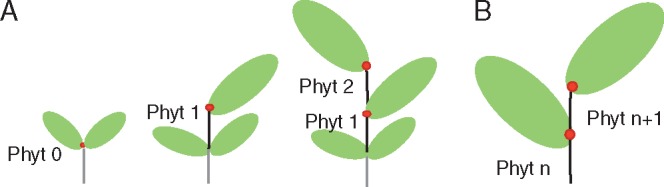
Background and aims: While the 'worldwide leaf economics spectrum' (Wright IJ, Reich PB, Westoby M, et al. 2004. The worldwide leaf economics spectrum. Nature : 821-827) defines mineral nutrient relationships in plants, no unifying functional consensus links size attributes. Here, the focus is upon leaf size, a much-studied plant trait that scales positively with habitat quality and components of plant size. The objective is to show that this wide range of relationships is explicable in terms of a seed-phytomer-leaf (SPL) theoretical model defining leaf size in terms of trade-offs involving the size, growth rate and number of the building blocks (phytomers) of which the young shoot is constructed.

Methods: Functional data for 2400+ species and English and Spanish vegetation surveys were used to explore interrelationships between leaf area, leaf width, canopy height, seed mass and leaf dry matter content (LDMC).

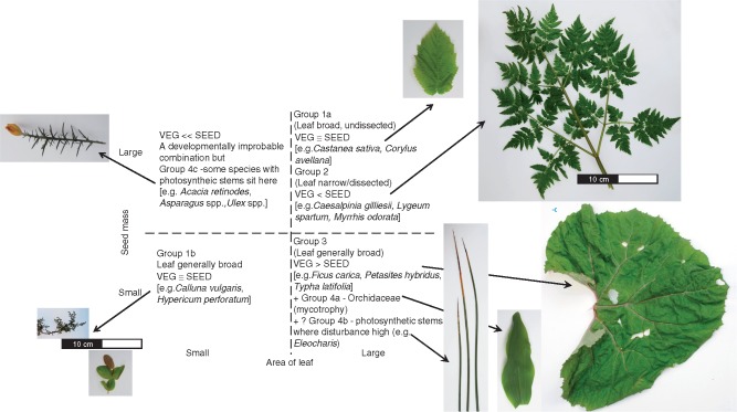
Key results: Leaf area was a consistent function of canopy height, LDMC and seed mass. Additionally, size traits are partially uncoupled. First, broad laminas help confer competitive exclusion while morphologically large leaves can, through dissection, be functionally small. Secondly, leaf size scales positively with plant size but many of the largest-leaved species are of medium height with basally supported leaves. Thirdly, photosynthetic stems may represent a functionally viable alternative to 'small seeds + large leaves' in disturbed, fertile habitats and 'large seeds + small leaves' in infertile ones.

Conclusions: Although key elements defining the juvenile growth phase remain unmeasured, our results broadly support SPL theory in that phytometer and leaf size are a product of the size of the initial shoot meristem (≅ seed mass) and the duration and quality of juvenile growth. These allometrically constrained traits combine to confer ecological specialization on individual species. Equally, they appear conservatively expressed within major taxa. Thus, 'evolutionary canalization' sensu Stebbins (Stebbins GL. 1974. Flowering plants: evolution above the species level . Cambridge, MA: Belknap Press) is perhaps associated with both seed and leaf development, and major taxa appear routinely specialized with respect to ecologically important size-related traits.

Keywords: Allometry; canopy height; canopy structure; evolutionary canalization; functional traits; leaf dry matter content; leaf width; photosynthetic stems; phylogeny; phytomer; seed–phytomer–leaf (SPL) theory; trade-offs.


Figures

F<sc>ig</sc>. 1.
Fig. 1.
Diagrammatic representation of phytomer growth. (A) Early stages of ‘juvenile growth’ (Phyt 0–2), with sequential phytomers increasing in size. (B) ‘Adult’ vegetative growth (Phyt n onwards), with sequential phytomers more or less even in size. Each phytomer consists of an internode (coloured black) and, above this, a node bearing a leaf (green) with an axillary bud (red).
F<sc>ig</sc>. 2.
Fig. 2.
Relationships between seed and leaf size for (A) a subset of 19 perennial species for which leaf size of juvenile (9-week-old) growth-room-grown plants (LAjuv) is additionally available, (B) species and major taxa and (C) vegetation. Here and in subsequent figures, data relate to LAdevel with, additionally, where different, statistics for LAmorph appended in parentheses. (Ai) LAjuv versus Seed M: log10LAjuv = 0·853log10Seed M + 2·643; r2 = 0·21 * (LAmorph: r2 = 0·19, P < 0·1). (Aii) LAjuv versus LAadult: log10LAjuv  = −0·103 log10LAadult2 + 1·122 log10LAadult + 0·162; r2 = 0·83 ***. (Aiii) LAadult versus Seed M: log10LAadult = 1·556 log10Seed M + 3·214; r2 = 0·48 *** (LAmorph: r2 = 0·43 **). (Bi) All species: log10LAdevel = 0·946log10Seed M + 2·919; r2 = 0·15, n = 2525 *** (LAmorph: r2 = 0·16 ***). (Bii) Mean values for families with ≥20 measured species. Regression using familial means (−): log10LAdevel = 0·997log10Seed M + 2·896; r2 = 0·30, n = 28 ** (LAmorph: r2 = 0·28 **). Families are grouped in relation to the statistical strength of r in intrafamilial correlations between LAdevel and Seed M. (Group 1) Intrafamilial correlation statistically significant at P < 0·05 (green dots): Amaryllidaceae, Apiaceae, Asteraceae, Brassicaceae, Boraginaceae, Caryophyllaceae, Euphorbiaceae, Fabaceae, Geraniaceae, Juncaceae, Lamiaceae, Malvaceae, Onagraceae, Poaceae, Ranunculaceae, Rubiaceae. (Group II) Blue dots (P < 0·1): Asparagaceae, Ericaceae, Primulaceae. (Group III) Red dots, ns; Amaranthaceae, Campanulaceae, Cyperaceae, Papaveraceae, Plantaginaceae, Polygonaceae, Rosaceae, Salicaceae. (Group IV) Red triangles, negative slope (P < 0·05): Cistaceae but log10LAdevel = −0·693√LDMC + 0·164Ht2 − 1·506Ht (r2 = 0·87, n = 20 ***) when other regression terms are added. Families abbreviated to their first three letters. (Biii) Life history groupings within Fabaceae. Test statistic for common slope across groups = 40·5, n = 196 ***: all slopes significantly different at P < 0·05. Annuals (blue dots, - - -): log10LAdevel = 0. 589log10Seed M + 2·220; r2 = 0·39, n = 118 ***; herbaceous perennials (green dots, – – –): log10LAdevel = 1·101log10Seed M + 2·309; r2 = 0·25, n = 49 ***; woody perennials (red dots, ): log10LAdevel = 1·678log10Seed M + 0·877; r2 = 0·34, n = 29 ***. (Ci) Central England: all quadrats: log10LAdevel = 1·069log10Seed M + 3·261; r2 = 0·22, n = 9050 *** (r2 = 0·21 ***). (Cii) Contrasted habitats: pasture (○): log10LAdevel = 1·947log10Seed M + 3·207; r2 = 0·28, n = 770 *** (LAmorph: r2 = 0·27 ***); woodland (black dots): log10LAdevel = 0·794log10Seed M + 3·188; r2 = 0·25, n = 1135 *** (LAmorph: r2 = 0·23 ***). (Ciii) North central Spain – all quadrats (grey dots): log10LAdevel = 1·038log10Seed M + 2·388; r2 = 0·02, n = 577 *** (r2 = 0·02 ***); artificial (open circles): log10LAdevel = 1·402log10Seed M + 2·541; r2 = 0·40, n = 130 ***; woodland (black dots): log10 LAdevel = –0·787log10Seed M – 0·665; r2 = 0·35, n = 91 ***. (North-east Spain, all quadrats: log10LAdevel = 0·963log10Seed M + 2·945; r2 = 0·05, n = 927 ***; not shown).
F<sc>ig</sc>. 3.
Fig. 3.
Relationships between leaf dry matter content (LDMC) and leaf size for (A) a subset of 19 perennial species with data for juvenile plants (B) species and (C) vegetation. (Ai) log10LAjuv = –0·701√LDMC + 5·897; r2 = 0·22 * (LAmorph: r2 = 0·07, ns). (Aii) log10LAadult = −1·278√LDMC + 9·151; r2 = 0·27 * (LAmorph: r2 = 0·15, P < 0·1). (B) log10LAdevel = −0·935log10√LDMC + 7·159; r2 = 0·014, n = 2448 *** (LAmorph: r2 = 0·011 ***). (Ci) Central England: log10LAdevel = − 0·827log10√LDMC + 6·750; r2 = 0·06, n = 9050 *** (LAmorph: r2 = 0·05 ***). (Cii) North central Spain: log10LAdevel = −0·397log10√LDMC + 4·428; r2 = 0·19, n = 577 *** (LAmorph: r2 = 0·20 ***). (North-east Spain: log10LAdevel = −0·094l√LDMC + 3·253; r2 = 0·02, n = 927 ***).
F<sc>ig</sc>. 4.
Fig. 4.
Relationships between canopy height class (Ht) and leaf size for (A) a subset of 19 species with data for juvenile plants, (B) species and (C) vegetation. (Ai) LAjuv = 0·536Ht + 0·428; r2 = 0·71 ***. (Aii) LAadult = 0·295Ht + 1·108; r2 = 0·72 *** (LAmorph: r2 = 0·69 ***). (B) LAdevel = −0·028Ht2 + 0·552Ht + 0·936; r2 = 0·30, n = 2448 *** (LAmorph: r2 = 0·29 *** (open circles identify median values). Additionally the relationships for small- and large-leaved species are illustrated by fitting a regression (dotted line) to the 5 and 95 percentiles for LAdevel at each height class (percentile5: LAdevel = 0·200Ht + 0·672; r2 = 0·96, n = 12 ***; percentile95: LAdevel = −0·038Ht2 + 0·643Ht + 1·785; r2 = 0·90, n = 12 ***). (Ci) Central England: LAdevel = −0·031Ht2 + 0·632Ht + 0·547; r2 = 0·36, n = 8972 *** (LAmorph: r2 = 0·37 ***). (Cii) North-east Spain: LAdevel = 0·347Ht + 0·997; r2 = 0·26, n = 927 *** (LAmorph: r2 = 0·24 ***). (North central Spain: LAdevel = 0·440Ht + 0·080; r2 = 0·15, n = 577 ***; not shown).
F<sc>ig</sc>. 5.
Fig. 5.
Relationships between leaf width and leaf shape for (A) angiosperm families and (B) vegetation in Central England. (Ai) Mean values for families. Families as in Fig. 2 abbreviated to the first three letters. (Aii) Two contrasted families, Boraginaceae (red dots, leaves ovate: log10LAfunct = 2·146log10LAdevel − 1·009; r2 = 0·78, n = 49 ***) and Apiaceae (black dots, leaves divided: log10LAfunct = 2·610log10LAdevel − 5·769; r2 = 0·13, n = 101 ***). Test statistic for common slope across groups 2·82, P < 0·1; Wald statistic shifts in elevation between groups 135·7 ***. (B) log10LAfunct = 2·470log10LAdevel − 3·119; r2 = 0·74, n = 9050 *** (LAmorph: r2 = 0·70 ***). Broken lines identify contours for leaf shape: ‘round’ (circular), ‘lanceolate’ (ellipse, eight times as long as broad) and ‘linear’ (32 times as long as broad). More complex leaf shapes (e.g. pinnately and palmately lobed leaves) are not included.
F<sc>ig</sc>. 6.
Fig. 6.
Comparison of functional traits of species with photosynthetic stems (stem) and mean trait values for the relevés with which they were associated (veg) in the SIVIM database (8000+ relevés with ‘photosynthetic stem’ species). Each point is a species. (A) Seed mass(stem) is a positive function of the mean values of their associated leafy vegetation for (i) LDMC (log10Seed Mstem = 3·533√LDMCveg − 16·120; r2 = 0·21, n = 24 *) and (ii) Ht (log10Seed Mstem = 1·982Htveg − 10·430; r2 = 0·30, n = 24 **). (B) Comparing functional traits (stem versus veg). (i) Seed M (log10Seed Mstem = 0·308log10Seed Mveg − 0·325; r2 = 0·52, n = 24 ***). (ii) Size of photosynthetic organ [log10Areastem = 0·311log10LAdevel_veg + 2·184; r2 = 0·23, n = 20 * (LAfunct: r2 = 0·26, n = 20 *)]. (iii) LDMC (√LDMCstem = 0·431√LDMCveg + 2·312; r2 = 0·61, n = 21 ***).
F<sc>ig</sc>. 7.
Fig. 7.
Emergent properties of SPL theory with particular reference to seed mass and leaf size and shape. (Groups 1a and 1b) Here, the relationship between seed mass and leaf size is broadly consistent with Fig. 2 and SPL theory. It illustrates a positive linear relationship between resource allocation to each seed reproduction unit [Seed M (≈ phytomer 0)] and that to each vegetative phytomer [LAdevel (≈ phytomer n)]. Thus, there appears to be a partial functional integration between the established vegetative and regenerative ‘seed’ phase of the plant’s life history. This integration may constrain divergence between seed and leaf size. (Group 2) Like group 1a but lamina elongated or dissected rather than broad and ovate. Although morphologically large, the leaves of Group 2 species are ‘functionally small’. Because of their narrow width, they have a much thinner boundary layer. For this grouping size traits conferring fitness during regeneration by seed appear to impact on trait expression in the vegetative phase. Thus, the regenerative ‘seed’ phase may be more important to survival than the established vegetative phase. (Group 3) Here, seed size is very small relative to leaf size (i.e. the converse of Group 2). Because of the long vulnerable juvenile phase from seedling to vegetative maturity, the expression of size-related traits appears primarily to reflect the functional requirements of the established vegetative phase. (Group 4) are functionally extreme. (Group 4a) Orchidaceae, with obligate mycotrophy, have minute dust-like seeds (mean value 0·004 mg, values from literature only) and a prolonged juvenile ‘protocorm’ stage. Mature plants tend to have large broad leaves (mean value from our data 1900 mm2; width 28 mm). (Group 4b, c) ‘Photosynthetic stem’ species. Representatives from each grouping are illustrated at a similar scale.

Similar articles

Cited by

References

    1. Aedo C. et al. 1980. onwards. Flora Iberica: plantas vasculares de la Península Ibérica e Islas Baleares. Madrid: Consejo Superior de Investigaciones Científicas.
    1. Angiosperm Phylogeny Group. 2016. An update of the Angiosperm Phylogeny Group classification for the orders and families of flowering plants: APG IV. Botanical Journal of the Linnean Society 181: 1–20.
    1. Barlow PW. 1994. Rhythm, periodicity and polarity as bases for morphogenesis in plants. Biological Reviews 69: 475–525.
    1. Baskin CC, Baskin JM.. 2014. Seeds. Ecology, biogeography, and evolution of dormancy and germination, 2nd edn.San Diego: Elsevier/Academic Press.
    1. de Bello F, Berg MP, Dias ATC, et al.2015. On the need for phylogenetic ‘corrections’ in functional trait-based approaches. Folia Geobotanica 50: 349–357.

Publication types