. 2017 Nov 10;62(23):8909-8923.
doi: 10.1088/1361-6560/aa93d1.

A 20-channel magnetoencephalography system based on optically pumped magnetometers

Affiliations

A 20-channel magnetoencephalography system based on optically pumped magnetometers

Amir Borna et al. Phys Med Biol. .

Abstract

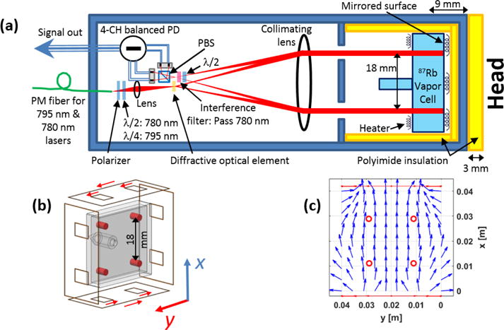
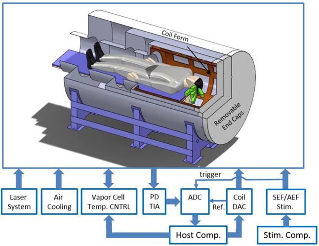
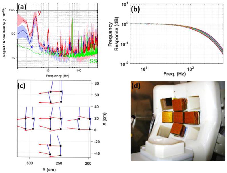
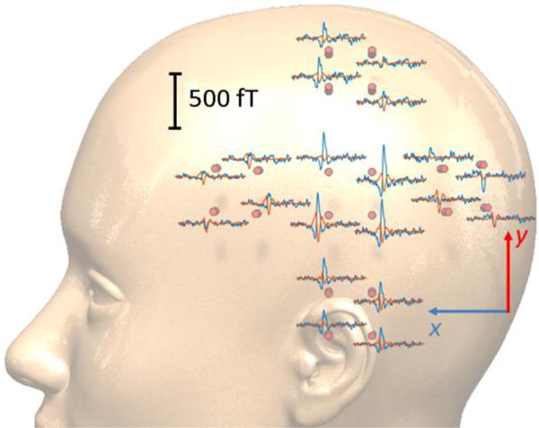
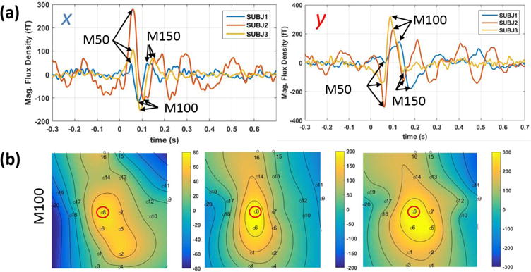
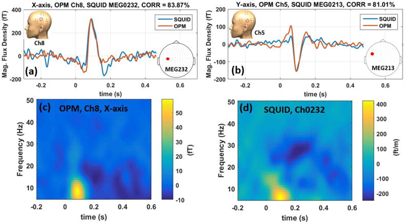
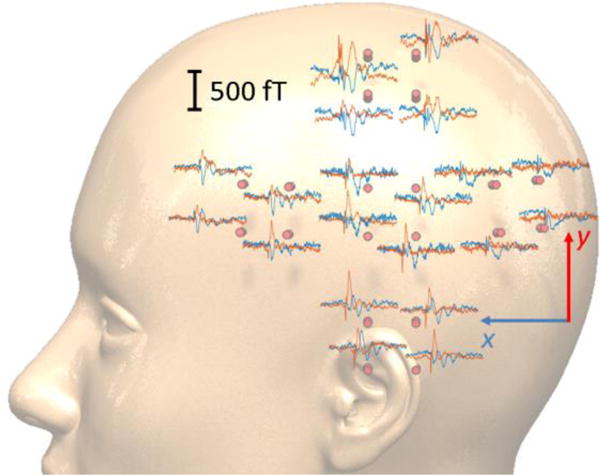
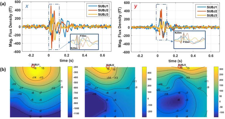
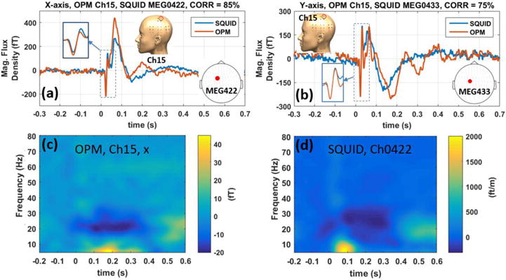
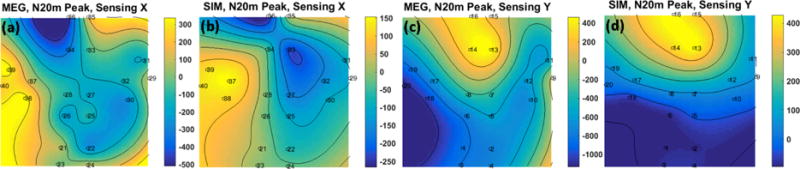
We describe a multichannel magnetoencephalography (MEG) system that uses optically pumped magnetometers (OPMs) to sense the magnetic fields of the human brain. The system consists of an array of 20 OPM channels conforming to the human subject's head, a person-sized magnetic shield containing the array and the human subject, a laser system to drive the OPM array, and various control and data acquisition systems. We conducted two MEG experiments: auditory evoked magnetic field and somatosensory evoked magnetic field, on three healthy male subjects, using both our OPM array and a 306-channel Elekta-Neuromag superconducting quantum interference device (SQUID) MEG system. The described OPM array measures the tangential components of the magnetic field as opposed to the radial component measured by most SQUID-based MEG systems. Herein, we compare the results of the OPM- and SQUID-based MEG systems on the auditory and somatosensory data recorded in the same individuals on both systems.


Figures

Figure 1
Figure 1
a) The OPM sensor’s schematic, b) a drawing of the on-sensor coils as they are positioned relative to the vapor cell (the red cylinders indicate the volume over which the magnetic field is measured, and the red arrows indicate the coils’ current flow to generate an x-axis field.), and c) the simulated magnetic field generated by the on-sensor coils. PBS: polarizing beam splitter; PM: polarization maintaining, PD: photodiode, λ/2: half wave plate, λ/4: quarter wave plate.
Figure 2
Figure 2
The MEG system block diagram. In the depiction of the cylindrical magnetic shield, a quarter section is removed to reveal the interior, showing the five OPM modules (green rectangles) placed against the head of a human subject. The overall length of the shield is 269 cm, and its external diameter is 140 cm. The diameter of the opening for the human subject is 60 cm. The diameter of the inner shield layer is 100 cm, and its length is 114 cm, excluding the 60-cm-diameter tube. PD TIA: the transimpedance amplifier which amplifies the currents coming from the sensors’ photo diodes; Temp. CNTRL: temperature control; ADC: analog-to-digital converter; DAC: digital-to-analog converter; SEF/AEF Stim.: refers to somatosensory/auditory evoked magnetic field stimulation; Ref.: reference for the lock-in amplifier.
Figure 3
Figure 3
a) The OPM sensors’ magnetic noise measured in the human-sized shield. The dark blue and red lines show the average noise for the array in the x and y directions, respectively. The shaded areas show the variation in noise across the channels. The green lines show the sensor noise measured in the small shield. b) The normalized frequency response of the OPM array’s 20 channels measured in the human-sized shield. c) The measured sense angle of the OPM array’s 20 channels for the x and y directions. d) The OPM array inside the human-sized shield.
Figure 4
Figure 4
The scalp level spatial topographies of the auditory evoked magnetic fields (AEF) measured using the presented 20-ch OPM array. Blue/red traces pertain to the x/y tangential components with 1 s of data shown. The middle sensor located above the ear shows the largest M100 component.
Figure 5
Figure 5
a) the time-domain auditory evoked magnetic fields time-locked to the standard tone for the y (left) and x (right) tangential components, b) fieldmap plots of the x-component of the magnetic field of the three subjects at the peak of M100. The channel plotted in (a) is circled in red on the fieldmap plots.
Figure 6
Figure 6
Comparing OPM vs. SQUID AEF data in time domain for x-axis (a) and y-axis (b). The SQUID data are scaled to match the amplitude of the OPM data. Time-frequency spectra of the OPM and SQUID AEF data are compared in (c) and (d) for the x-axis modulation. These figures show excellent agreement between the SQUID and OPM array in both time and frequency domains.
Figure 7
Figure 7
Measured single-trial somatosensory evoked magnetic fields (SEF) using the OPM array before (a) and after (b) applying independent component analysis (ICA). The zigzag features visible in raw epochs (a) pertain to the MCG which are removed using ICA. The single-trial time domain waveforms of raw and processed epochs are compared in (c). The inset highlights the sensor location.
Figure 8
Figure 8
Measured time-locked somatosensory evoked magnetic fields (SEF) before (a) and after (b) applying independent component analysis (ICA). ICA removes the low frequency component peaking at 100 ms and reaching as large as 7 pT. The blue traces represent the x-axis and the red traces are the y-axis component. The black trace in (a) is from the control experiment showing that the observed M100 is not present when the electrodes are slightly off the median nerve.
Figure 9
Figure 9
The scalp level spatial topographies of the somatosensory evoked magnetic fields (SEF) measured using the 20-channel OPM array. Blue/red traces pertain to the x/y tangential components. The sensors located on top of the head show the largest N20m/P30m components.
Figure 10
Figure 10
a) The somatosensory evoked magnetic fields (SEF), in time-domain for the x (left) and y (right) tangential components; b) the field maps of three subjects for the y-axis at the peak of N20m. The channel shown in (a) is encircled in read on the fieldmap plots.
Figure 11
Figure 11
Comparing OPM vs SQUID SEF data in time domain for x (a) and y (b) tangential components. Time-frequency spectrum of the OPM’s x-axis and SQUID SEF data are compared in (c) and (d) respectively.
Figure 12
Figure 12
Comparing the fieldmaps generated from the SEF MEG data at the peak of N20m, (a) and (c), captured by the presented OPM system and (b) and (d), the simulation based on the dipole fit from the SQUID measurement/analysis; the contours have the unit of fT.

References

    1. Cohen D. MAGNETOENCEPHALOGRAPHY - EVIDENCE OF MAGNETIC FIELDS PRODUCED BY ALPHA-RHYTHM CURRENTS. Science. 1968;161(3843):784. &. - PubMed
    1. Hämäläinen M, et al. Magnetoencephalography–theory, instrumentation, and applications to noninvasive studies of the working human brain. Rev Mod Phys. 1993;65(2):413–497.
    1. Iivanainen J, Stenroos M, Parkkonen L. Measuring MEG closer to the brain: Performance of on-scalp sensor arrays. NeuroImage. 2017;147:542–553. - PMC - PubMed
    1. Boto E, et al. On the Potential of a New Generation of Magnetometers for MEG: A Beamformer Simulation Study. Plos One. 2016;11(8) - PMC - PubMed
    1. Xia H, et al. Magnetoencephalography with an atomic magnetometer. Applied Physics Letters. 2006;89(21):211104.

LinkOut - more resources