Color opponency: tutorial

Abstract

In dialogue, two color scientists introduce the topic of color opponency, as seen from the viewpoints of color appearance (psychophysics) and measurement of nerve cell responses (physiology). Points of difference as well as points of convergence between these viewpoints are explained. Key experiments from the psychophysical and physiological literature are covered in detail to help readers from these two broad fields understand each other's work.

Fig. 1

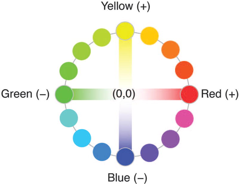
Color opponent axes. Hering declared red and green to be opponent colors represented along a single axis. Here, positive values on the axis are reddish, negative values are greenish, and zero represents a hue that has no redness or greenness at all—that is, unique blue, unique yellow, or white. Hering also proposed a second axis running from yellow (positive) to blue (negative), with zero for hues that have no yellowness or blueness (so unique red, unique green, or white). Any hue can be represented by two coordinate values, one on each axis. Orange, for example, has a positive value on both axes; aqua, composed of both greenness and blueness, has a negative value on both axes. White has zero on both axes (no trace of redness, greenness, yellowness, or blueness).

Fig. 2

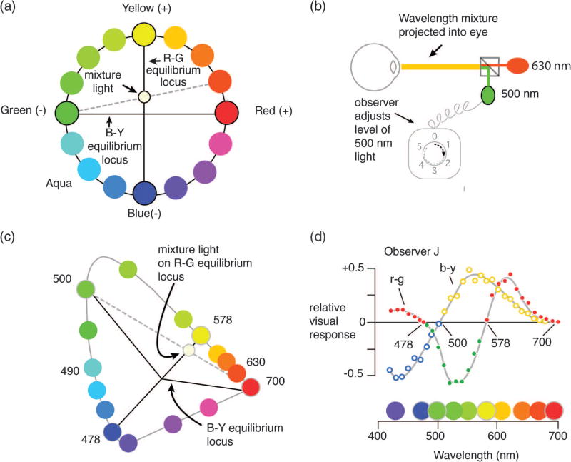
How to use color mixtures to characterize opponent-color mechanisms. (a) Hues that do not lie on the opponent axes have both red–green and blue–yellow components. In this case, orange has red and yellow components. By adding 500 nm (“green”) to the orange hue its reddish component can be canceled (i.e., bringing the mixture light to the R–G equilibrium locus). (b) Mixing spectral lights. The observer views a mixture of 630 nm plus a greenish-appearing wavelength (here, 500 nm), and adjusts the level of the 500 nm light until the mixture appears neither reddish nor greenish. (c) A representation of the Jameson and Hurvich color cancellation experiment in CIE space. Repeating the chromatic cancellation for wavelengths above 578 nm quantifies the redness in each of these wavelengths. (d) The resulting measurements can be plotted together as a function of all the physical wavelengths in the visible spectrum (see text).

Fig. 3

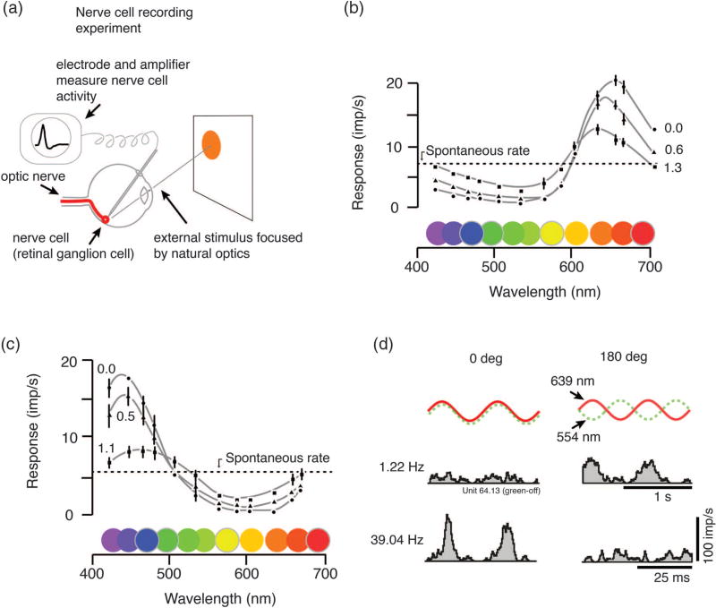
Physiological measurement of opponency. (a) Opponency defined by nerve cell recording. The visual system of an anaesthetized monkey responds to brief pulses of light presented on a stimulus screen. The small electrical signals (action potentials) from these cells are picked up by an electrode and amplified. (b) These famous recordings by De Valois and colleagues show responses of single nerve cells in monkey visual system to lights at different wavelengths. Here the opponent process is revealed as the cell is excited by some wavelengths (in this case, long wavelengths) and inhibited by others (that is, the spike rate falls below the maintained rate). Measurements were taken at three steps of brightness attenuation, showing that the opponent characteristic does not depend heavily on brightness. (c) Other cells show blue–yellow opponent property. (d) Opponency can also be measured by responses to a mixture of wavelengths projected into the eye. The frequency of action potentials is measured as a function of time relative to the stimulus modulation. If the response to in-phase modulation (0 deg phase difference, left column) is less than the response to out-of-phase modulation (180 deg phase difference, right column), we know that something in the retina has “subtracted” the neural response to 554 nm (“green”) light from the response to 639 nm (“red”) light (upper histograms). The process can be studied in detail by changing the frequency and phase of light modulation (lower histograms). Panels (b) and (c) modified from [12]. Panel (d) modified from Solomon et al. (2005) [13].

Fig. 4

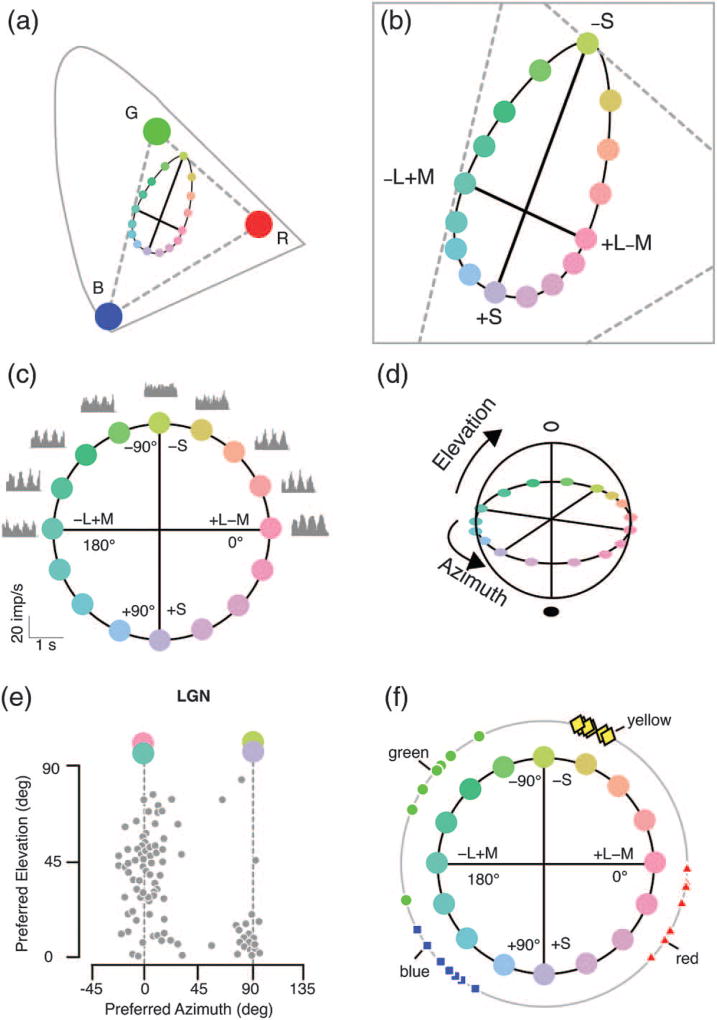
Cone opponency defined physiologically by chromatic cardinal axes in experiments by Derrington and colleagues. (a) Projection of the stimulus set onto the CIE axes. Broken lines show the range of colors that lie within the monitor gamut. (b) Enlarged view of part of this space. Thick solid lines show two cardinal exchange axes producing selective modulation of S cones and out-of-phase modulation of M and L cones at constant luminance. Intermediate modulation directions form an ellipse in this space. (c) Here the space is reformed into a circle with cone excitation azimuth. Gray profiles show response modulation of a single nerve cell along different color modulation directions (four cycles of modulation are shown). Note that the cell is modulated maximally by exchange along the L–M axis (0–180 deg), and shows no modulation (response “null”) along the S-cone axis (90 to −90 deg). (d) A third axis (elevation) is defined by in-phase modulation of S, M, and L cones. (e) Two clusters of cells are present in monkey lateral geniculate nucleus (LGN) with preferred azimuth close to zero (L–M) or 90 (S) deg. The L–M cells prefer a combination of luminance and color exchange (elevations around 45 deg), whereas the S cells prefer near-equiluminant color exchange. (f) Unique hues (outer circle) do not align with the cardinal color axes. The points show unique hue settings made on the circumference of an S versus ML cone space circle by seven observers. Note that the settings do not align with the L–M or S axis. Note also the differences in unique hue position among observers, with little variation in unique yellow but wide variation in position of unique blue, red, and green. Data in panels (c) and (e) redrawn from [40]. Data in panel (f) redrawn from [35].

Fig. 5

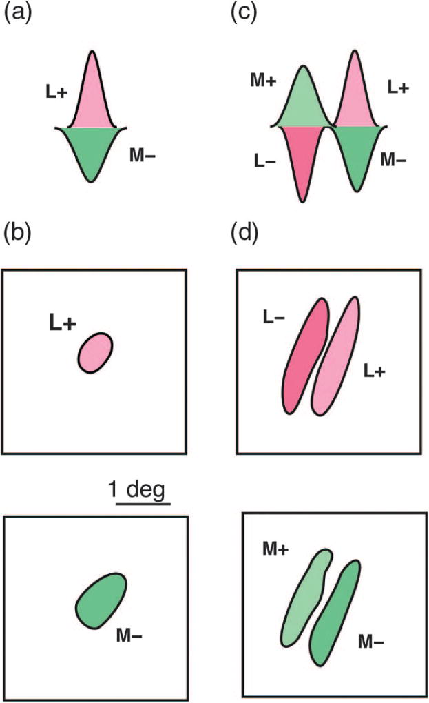
Spatial and chromatic opponent receptive fields. (a) Schematic spatial sensitivity profile of a single-opponent receptive field receiving excitatory input (L+) from long-wave sensitive cones, and inhibitory input (M−) from middle-wave sensitive cones. (b) The receptive field projection of a single-opponent field shows approximately overlapping and circularly symmetric cone-opponent inputs. (c) Schematic spatial sensitivity profile of a double-opponent receptive field. Here the receptive field comprises two opponent sub-regions which are spatially offset. (d) The receptive field projection of a double-opponent field shows complementary, orientation-selective sub-regions which produce both spatial and chromatic selectivity. Modified from [53].

References

-
- Hering E. Zur Lehre vom Lichtsinn. Gerald u. Söhne; 1878. Grundzüge einer Theorie des Farbensinnes (originally published in 1874) pp. 107–141.
- Turner RS. Vision studies in Germany: Helmholtz versus Hering. Osiris. 1993;8:80–103. - PubMed
- Young T. The Bakerian lecture: on the theory of light and colours. Philos. Trans. R. Soc. London. 1802;92:12–48.
- Mollon JD. The origins of modern color science. In: Shevell SK, editor. The Science of Color. Optical Society of America/Elsevier; 2003. pp. 1–39.
- Helmholtz H. In: Helmholtz’s Treatise on Physiological Optics. Southall JPC, editor. 1–2 Dover: 1962.
Grants and funding
LinkOut - more resources
Full Text Sources
Other Literature Sources