. 2017 Dec;207(4):1591-1619.
doi: 10.1534/genetics.117.300417. Epub 2017 Oct 18.

Distinguishing Among Modes of Convergent Adaptation Using Population Genomic Data

Affiliations

Distinguishing Among Modes of Convergent Adaptation Using Population Genomic Data

Kristin M Lee et al. Genetics. 2017 Dec.

Abstract

Geographically separated populations can convergently adapt to the same selection pressure. Convergent evolution at the level of a gene may arise via three distinct modes. The selected alleles can (1) have multiple independent mutational origins, (2) be shared due to shared ancestral standing variation, or (3) spread throughout subpopulations via gene flow. We present a model-based, statistical approach that utilizes genomic data to detect cases of convergent adaptation at the genetic level, identify the loci involved and distinguish among these modes. To understand the impact of convergent positive selection on neutral diversity at linked loci, we make use of the fact that hitchhiking can be modeled as an increase in the variance in neutral allele frequencies around a selected site within a population. We build on coalescent theory to show how shared hitchhiking events between subpopulations act to increase covariance in allele frequencies between subpopulations at loci near the selected site, and extend this theory under different models of migration and selection on the same standing variation. We incorporate this hitchhiking effect into a multivariate normal model of allele frequencies that also accounts for population structure. Based on this theory, we present a composite-likelihood-based approach that utilizes genomic data to identify loci involved in convergence, and distinguishes among alternate modes of convergent adaptation. We illustrate our method on genome-wide polymorphism data from two distinct cases of convergent adaptation. First, we investigate the adaptation for copper toxicity tolerance in two populations of the common yellow monkey flower, Mimulus guttatus We show that selection has occurred on an allele that has been standing in these populations prior to the onset of copper mining in this region. Lastly, we apply our method to data from four populations of the killifish, Fundulus heteroclitus, that show very rapid convergent adaptation for tolerance to industrial pollutants. Here, we identify a single locus at which both independent mutation events and selection on an allele shared via gene flow, either slightly before or during selection, play a role in adaptation across the species' range.

Keywords: coalescent theory; composite likelihood; convergent adaptation; genetic hitchhiking; positive selection.


Figures

Figure 1
Figure 1
Present day population allele frequencies at a given neutral locus (x1x4 for populations 1–4, respectively) are derived from ancestral allele frequency ε. Each population has a coancestry coefficient proportional to the amount of drift experienced since the split from the ancestral population. f11 is shown for population 1. Here, populations 1 and 2, and 3 and 4 share drift relative to the ancestral population, and have nonzero coancestry coefficients f12 and f34, respectively. Blue diamonds represent the novel selective environment, and red circles the ancestral environment. Note that branch lengths are not proportional to time in generations (unless there is no migration and the amount of drift is small).
Figure 2
Figure 2
Trajectories of the beneficial allele (red) for the three modes of convergent adaptation. Populations i and j are under selection with present-day allele frequencies xi and xj at a neutral locus, derived from an ancestral population with allele frequency ε. The populations share some amount of drift proportional to fij before reaching the ancestral population. (A) Independent mutations model. Beneficial mutations, indicated by the orange triangles, occur independently in the selected populations after they have become isolated. Selection begins, indicated by the blue triangles, once the beneficial allele is present in the population. The beneficial allele sweep to fixation in ts generations. (B) Standing variant model. The beneficial allele is standing at frequency g in the ancestral population. After the selected populations split, it is still standing at frequency g for t generations prior to the onset of selection. (C) Migration model. The beneficial allele arises in population i and begins sweeping in population i. Meanwhile, there is a continuous low level of migration from population i into population j. The beneficial allele establishes in j after δ generations, where it is swept to fixation in ts generations.
Figure 3
Figure 3
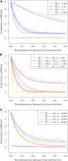
We calculated the average coancestry coefficient values across 1000 runs of simulations for each of 100 bins of distance away from the selected site to compare our simulation results (dashed lines) to our theoretical expectations (solid lines). (A) Average coancestry coefficients under the independent mutations model (Ne=100,000) within a selected population (population 2) with varying s. Also shown is the coancestry coefficient between selected populations which in this case is 0, the neutral expectation. (B) Coancestry coefficients under the standing variation model between selected populations with varying amount of time beneficial allele has been independently standing in populations (t). The coancestry coefficient within a single population is also shown for t=50. For all, Ne=10,000, g=0.001, and s=0.01. (C) Coancestry coefficients under the migration model, within both selected populations (source population 2 and recipient population 3) as well as between source and recipient (2,3) and between recipient and a nonselected population (1,3). Here, we show one set of parameters (s=0.01, m=0.001,and Ne=10,000), as estimates do not vary dramatically with changing m (see Figure S2 in File S1).
Figure 4
Figure 4
MCLEs calculated under model used for simulation. We vary the true value of the parameter used for simulations along the x-axis, and show the MCLE for each of 100 simulations (points). Crossbars indicate first and third quartiles with second quartiles (medians) as the horizontal line. The true values of the parameters are marked with dashed, black lines. (A) MCLE of the location of selected site for 100 simulations under the independent mutation model (10 chromosomes per population, Ne = 100,000, and s = 0.05). (B) MCLE of the strength of selection (s) for 100 simulations under the independent mutation model (10 chromosomes per population, Ne = 100,000). (C) MCLE of the standing time (t) for 100 simulations under the standing variant model (10 chromosomes per population, Ne = 10,000, s = 0.01, and g = 0.001). For scale, we left out estimates of t> 15,000 (2, 9, and 21 data points when ttruth = 500, 1000, and 5000, respectively.)
Figure 5
Figure 5
Composite log-likelihood surface of the strength of selection (s) and the frequency of standing variant (g) for three simulations (with Ne = 10,000, t = 500, g = 0.001, and s=0.01) to exemplify confounding of s and g under the standing variant model. Blue diamond pluses represent the true location of the parameters used for simulation. Blue circles represent MCLE.
Figure 6
Figure 6
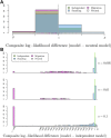
Histograms of the differences in maximum composite log-likelihoods calculated under a given model relative to the true model used for 100 simulations. Parameter values used to simulate are noted, varying along the vertical dimension. Values <0, marked with solid line, indicate the true model has a higher maximum composite likelihood than alternative model. Conversely, values >0 indicate the alternative, incorrect model of convergence has a higher composite log-likelihood than the true model. True models: (A) Differences in maximum composite log-likelihoods under models relative to neutral model. (B) Differences in maximum composite log-likelihoods under models relative to independent mutations model with Ne=100,000. (C) Differences in maximum composite log-likelihoods under models relative to standing variation model with Ne=10,000, s=0.01, and g=0.001. (D) Differences in maximum composite log-likelihoods under models relative to migration model with Ne=10,000 and s=0.01.
Figure 6
Figure 6
Histograms of the differences in maximum composite log-likelihoods calculated under a given model relative to the true model used for 100 simulations. Parameter values used to simulate are noted, varying along the vertical dimension. Values <0, marked with solid line, indicate the true model has a higher maximum composite likelihood than alternative model. Conversely, values >0 indicate the alternative, incorrect model of convergence has a higher composite log-likelihood than the true model. True models: (A) Differences in maximum composite log-likelihoods under models relative to neutral model. (B) Differences in maximum composite log-likelihoods under models relative to independent mutations model with Ne=100,000. (C) Differences in maximum composite log-likelihoods under models relative to standing variation model with Ne=10,000, s=0.01, and g=0.001. (D) Differences in maximum composite log-likelihoods under models relative to migration model with Ne=10,000 and s=0.01.
Figure 7
Figure 7
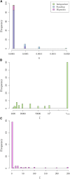
Histograms of MCLE for parameters estimated under incorrect models. (A) Histogram of MCLE of the strength of selection (s) under all convergent models where the neutral model is true model used for simulations. (B) Histogram of MCLE of the standing time (t) under standing variant model where the independent mutation model is true model used for simulations (s = 0.01 and Ne = 100,000). (C) Histogram of MCLE of the standing time (t) under standing variant model where the migration model is true model used for simulations (m = 0.001, s = 0.01, and Ne = 10,000).
Figure 8
Figure 8
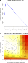
Inference results for M. guttatus copper tolerance adaptation on Scaffold8. (A) Composite log-likelihood ratio of given model relative to neutral model of no selection as a function of the proposed selected site. We show likelihoods for the standing-source model maximizing over possible sources, but all results can be seen in Figure S7a in File S1. (B and C) MCLE of parameters in standing variation model with position 308,503 as selected site. (B) Profile composite log-likelihood surface for minimum age of standing variant, maximizing over other parameters, with peak at 646 generations (C) Composite log-likelihood surface for strength of selection vs. frequency of standing variant. Blue circle represents point estimate of joint MCLE (s^ = 0.034 and g^=107). t is held constant at MCLE of 646 generations.
Figure 9
Figure 9
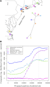
(A) Map of sampled killifish populations with phylogenetic tree, showing that the southern pair (T4, S4) are more distant than other populations. Tree is estimated from genome-wide biallelic SNP frequencies using Phylogeny Inference Package (PHYLIP) Gene Frequencies and Continuous Characters Maximum Likelihood (CONTML) module [see Reid et al. (2016) for more information]. (B) Inference results for Fundulus heteroclitus pollutant tolerance adaptation on Scaffold9893. Composite log-likelihood ratio of given model relative to neutral model of no selection as a function of the proposed selected site. Closed points represent models where all four populations have same convergent mode, while open points represent Southern population (T4) having an independent mutation at the proposed selected site. We show likelihoods maximizing over possible sources, but all results can be seen in Figure S9 in File S1. The AIP locus position is marked by the vertical, dashed gray lines.
Figure 10
Figure 10
The composite log-likelihood surfaces for the parameters for F. heteroclitus convergent data in combined standing variation, and independent sweep model with position 1,961,198 on Scaffold9893 as selected site and population T3 as source. (A) Profile composite log-likelihood surface for minimum age of standing variant, maximizing over other parameters, showing the beneficial allele has been standing for a very short amount of time in our three northern populations (eight generations). (B) Composite log-likelihood surface for strength of selection vs. frequency of standing variant. Blue circle represents point estimate of joint MCLE (s^ = 0.3, g^=108). t is held at MCLE of eight generations.
Figure 11
Figure 11
Trajectories of the beneficial allele (red) for the standing variant model with a source population. Populations l and i are under selection with present-day allele frequencies xl and xi at a neutral locus, derived from an ancestral population with allele frequency ε. The populations share some amount of drift proportional to fil before reaching the ancestral population. The beneficial allele is standing at frequency g in the source population, l. It migrates into population i from l, where it is standing at frequency g for t generations prior to the onset of selection, indicated by the blue triangles.

Similar articles

Cited by

References

    1. Arendt J., Reznick D., 2008. Convergence and parallelism reconsidered: what have we learned about the genetics of adaptation? Trends Ecol. Evol. 23: 26–32. - PubMed
    1. Aubury L. E., 1902. The Copper Resources of California (No. 23). Superintendent State Printing, Sacramento, CA.
    1. Barrett R. D., Schluter D., 2008. Adaptation from standing genetic variation. Trends Ecol. Evol. 23: 38–44. - PubMed
    1. Barton N., 1998. The effect of hitch-hiking on neutral genealogies. Genet. Res. 72: 123–133.
    1. Barton N., Bengtsson B. O., 1986. The barrier to genetic exchange between hybridising populations. Heredity 57: 357–376. - PubMed

Publication types