Development of a Bayesian Estimator for Audio-Visual Integration: A Neurocomputational Study

Abstract

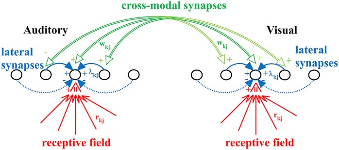
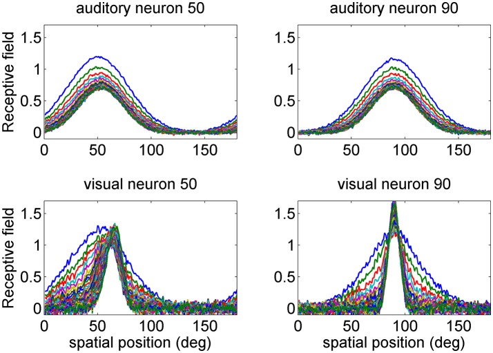
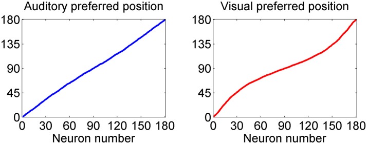
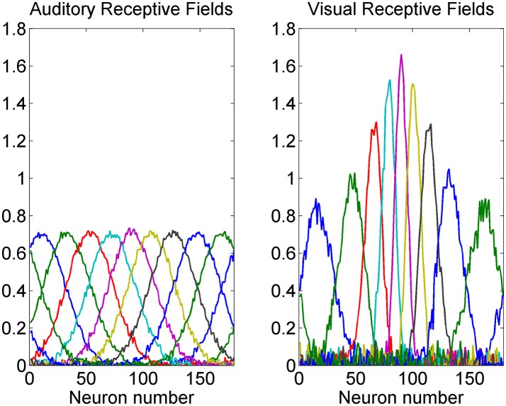
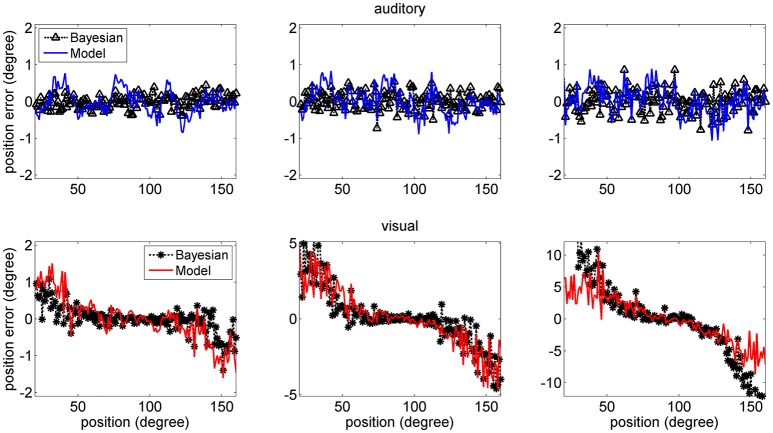
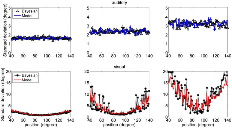
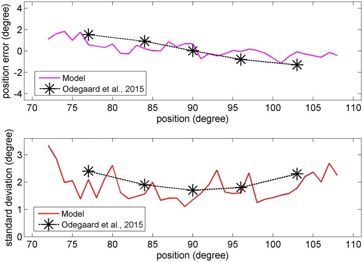
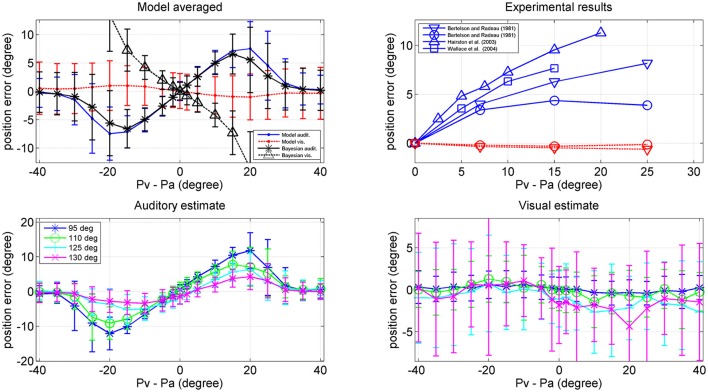
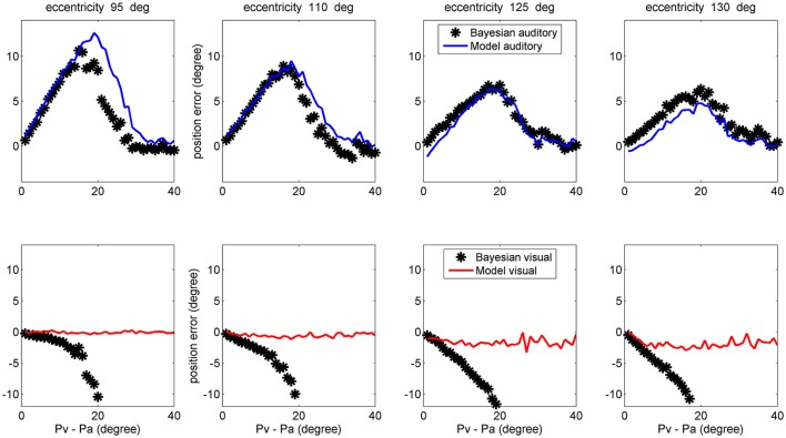
The brain integrates information from different sensory modalities to generate a coherent and accurate percept of external events. Several experimental studies suggest that this integration follows the principle of Bayesian estimate. However, the neural mechanisms responsible for this behavior, and its development in a multisensory environment, are still insufficiently understood. We recently presented a neural network model of audio-visual integration (Neural Computation, 2017) to investigate how a Bayesian estimator can spontaneously develop from the statistics of external stimuli. Model assumes the presence of two unimodal areas (auditory and visual) topologically organized. Neurons in each area receive an input from the external environment, computed as the inner product of the sensory-specific stimulus and the receptive field synapses, and a cross-modal input from neurons of the other modality. Based on sensory experience, synapses were trained via Hebbian potentiation and a decay term. Aim of this work is to improve the previous model, including a more realistic distribution of visual stimuli: visual stimuli have a higher spatial accuracy at the central azimuthal coordinate and a lower accuracy at the periphery. Moreover, their prior probability is higher at the center, and decreases toward the periphery. Simulations show that, after training, the receptive fields of visual and auditory neurons shrink to reproduce the accuracy of the input (both at the center and at the periphery in the visual case), thus realizing the likelihood estimate of unimodal spatial position. Moreover, the preferred positions of visual neurons contract toward the center, thus encoding the prior probability of the visual input. Finally, a prior probability of the co-occurrence of audio-visual stimuli is encoded in the cross-modal synapses. The model is able to simulate the main properties of a Bayesian estimator and to reproduce behavioral data in all conditions examined. In particular, in unisensory conditions the visual estimates exhibit a bias toward the fovea, which increases with the level of noise. In cross modal conditions, the SD of the estimates decreases when using congruent audio-visual stimuli, and a ventriloquism effect becomes evident in case of spatially disparate stimuli. Moreover, the ventriloquism decreases with the eccentricity.

Keywords: multisensory integration; neural networks; perception bias; prior probability; ventriloquism.

Figure 1

The neural network used in the present work. Each neuron accomplishes the scalar product of the external stimulus and its receptive field (r_kj), but also receives lateral synapses (λ_kj) from other neurons of the same modality, and cross-modal synapses (w_kj) from neurons of the other modality. Synapses r_kj and w_kj are trained with the adopted learning rule.

Figure 2

Examples of the progressive shrinking of the receptive fields (RFs) during training. The figures illustrate the RFs of two exemplary neurons in the auditory network (Upper) and in the visual network (Bottom). The initial preferred positions of these neurons were at 50 and 90 deg (blue lines). It is worth noting that, at the end of training (green lines), the visual RFs are more tuned than the auditory ones, reflecting the more precise spatial localization of the inputs. Moreover, the RF of the visual neuron at initial position 50 deg shifts toward the fovea, as a consequence of the higher prior probability of central visual stimuli. The auditory RFs do not exhibit an appreciable shift.

Figure 3

Distribution of the preferred positions for all 180 auditory (Left) and visual (Right) neurons after training. The distribution of auditory neurons is linear, i.e., the RFs are uniformly distributed, reflecting the uniform unisensory prior. Conversely, the distribution of the visual neurons is denser toward the fovea, reflecting the Gaussian distribution of the prior (with more visual stimuli at the center, and less at the periphery).

Figure 4

Exempla of auditory (Left) and visual (Right) RFs after training. We showed the RFs of neurons with initial preferred positions from 10 to 170 deg with a 20 deg step. It is evident that the visual RFs are denser and more precise close to the fovea.

Figure 5

Example of cross-modal synapses after training. Each curve represents the synapses that reach one auditory neuron (Left) or one visual neuron (Right) from all 180 neurons in the other modality. We showed neurons with initial preferred positions from 10 to 170 deg with a 20 deg step. It is worth noting that auditory neurons receive stronger cross-modal synapses when they are placed toward the fovea, whereas visual neurons receive stronger cross-modal synapses when placed at the periphery. Moreover, each neuron receives synapses only from other neurons with similar preferred positions. These patterns reflect the prior on the proximity of visual and auditory positions in cross-modal stimulation, and the prior on the higher frequency of visual stimuli at the fovea, and scarce frequency of visual stimuli at the periphery.

Figure 6

Position errors for the model estimates (Equation 15) for the auditory (Upper: blue lines) and visual (Bottom: red lines) stimuli in unisensory conditions, as a function of the true stimulus position. Each point is the average of one hundred trials. The left column has been obtained using a SD of noise as low as 33% of the maximum input. The middle and right columns have been obtained with a SD of noise as high as 50 and 66% of the maximum input, respectively. In these figures, the peripheral space is not shown, due to the large SD of the visual estimates (i.e., visual estimates are nor reliable there). It is worth noting the bias of visual estimates toward the fovea, reflecting the non-uniform distribution of the unisensory visual inputs. Moreover, this bias increases with the superimposed noise. Results are compared with those obtained with the Bayesian estimator (Equation 16, black symbols).

Figure 7

SD deviations for the auditory (Upper: blue lines) and visual (Bottom: red lines) estimates in unisensory conditions, as a function of the true stimulus position. Each point was computed from one hundred trials. Results have been obtained from the same simulation data as in Figure 6. It is worth noting that the SD of all estimates increases with the noise level (from left to right, 33, 50, and 66%). Moreover, the visual estimates have smaller SD close to the fovea compared with the auditory estimates (0.8 vs. 1.5 deg, left column; 1.2 vs. 2.4 deg middle column; 2 vs. 3.5 deg right colum), but their SDs increase at the periphery. Results are compared with those obtained with the Bayesian estimator (Equation 16, black symbols).

Figure 8

Upper: Comparison between the visual estimation bias computed with the model with 66% of superimposed noise (red line), and that reported by Odegaard et al. (2015) (black symbols). Bottom: Comparison between the visual SD computed with the model with 50% of superimposed noise (red line), and that reported by Odegaard et al. (2015) (black symbols).

Figure 9

Position errors (Upper), and SD of the estimates (Bottom) computed with the model (Equation 15) for the auditory (Left: blue lines) and visual (Right: red lines) stimuli in cross-modal conditions, with the two stimuli at the same position. Each point is the average of one hundred trials. The SD of noise was 50% of the maximum input. It is worth noting that the bias of the visual estimate and its SD are smaller than in the unisensory case. Moreover, the SD of the auditory estimate is significantly smaller than in the unisensory case. Black points are the results of the theoretical Bayesian estimator.

Figure 10

Upper left: Ventriloquism effect simulated with the network during cross-modal trials. Cross modal trials were performed, by moving the visual stimulus from position 40 deg to position 140 deg and, at each visual position, adding a second auditory stimulus with a shift in the range from –40 to + 40 deg from the visual one. One hundred trials were performed at each condition, with 50% noise. Results are averaged over all the 100 positions and over all 100 trials per each shift. The x-axis represents the audio-visual distance (where positive values indicate that the visual stimulus is placed on the right), the y-axis is the perceived error (estimated position minus true position): auditory perception, continuous blue line; visual perception, dotted red line. The black lines represent the error of the Bayesian estimate (*auditory, Δ visual) averaged over the same trials. Bars denote standard deviations. Upper right: Behavioral data from Hairston et al. (2003) Δ, Wallace et al. (2004) □, Bertelson and Radeau (1981) ∇, and o. Bottom: Auditory (Left) and (Right) visual position errors evaluated with the model when the visual stimulus was fixed at position 95 deg (blue), 110 deg (green), 125 deg (cyan), and 130 deg (magenta). The auditory ventriloquism effect decreases with the azimuthal position.

Figure 11

Comparison between the ventriloquism effect simulated with the network and predictions of the Bayesian estimator, evaluated at different azimuthal positions for the visual stimulus (first column 95 deg; second column: 110 deg; third column: 125 deg; fourth column: 130 deg). Upper: The auditory bias decreases with the visual azimuthal coordinate, both in the model (blue lines) and in the Bayesian estimator (black). Bottom: The model exhibits negligible visual bias (red lines), whereas the Bayesian estimator exhibits a significant visual bias (black) at large audio-visual shifts (visual shifts more negative than 10 deg, occurring at audio-visual disparity lager than 20 deg, are not reported since clearly unrealistic). A 50% noise was used during these trials.

References

1. Alais D., Burr D. (2004). The ventriloquist effect results from near-optimal bimodal integration. Curr. Biol. 14, 257–262. 10.1016/j.cub.2004.01.029 - DOI - PubMed
1. Aslin R. N., Newport E. L. (2012). Statistical learning: from acquiring specific items to forming general rules. Curr. Dir. Psychol. Sci. 21, 170–176. 10.1177/0963721412436806 - DOI - PMC - PubMed
1. Bertelson P., Radeau M. (1981). Cross-modal bias and perceptual fusion with auditory-visual spatial discordance. Percept. Psychophys. 29, 578–584. 10.3758/BF03207374 - DOI - PubMed
1. Birch E., Gwiazda J., Bauer J., Naegele J., Held R. (1983). Visual acuity and its meridional variations in children aged 7–60 months. Vis. Res. 23, 1019–1024. 10.1016/0042-6989(83)90012-3 - DOI - PubMed
1. Blakemore C., Cooper G. F. (1970). Development of the brain depends on the visual environment. Nature 228, 477–478. 10.1038/228477a0 - DOI - PubMed
LinkOut - more resources