Multiscale 3D Genome Rewiring during Mouse Neural Development

Abstract

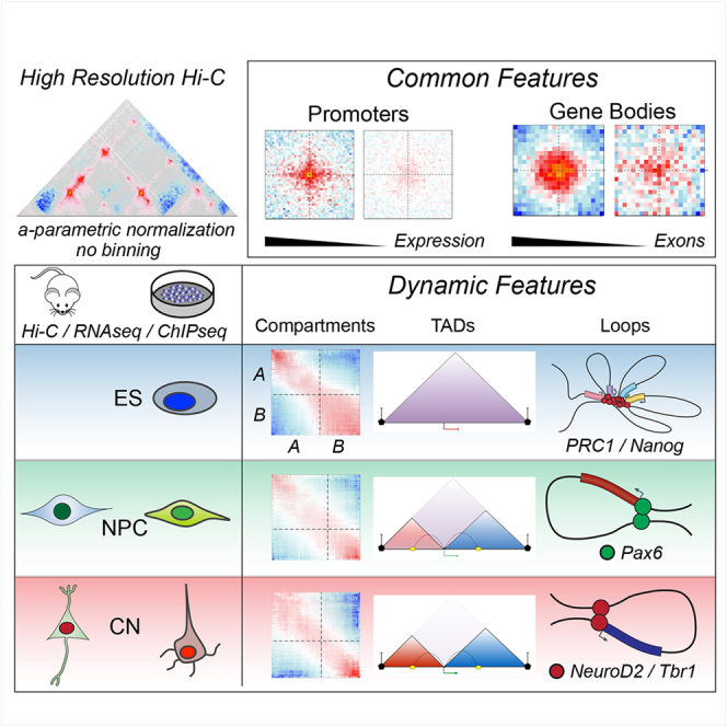
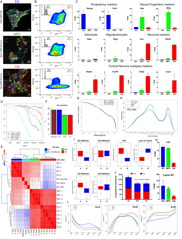
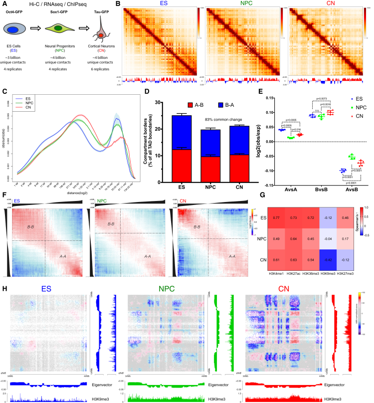
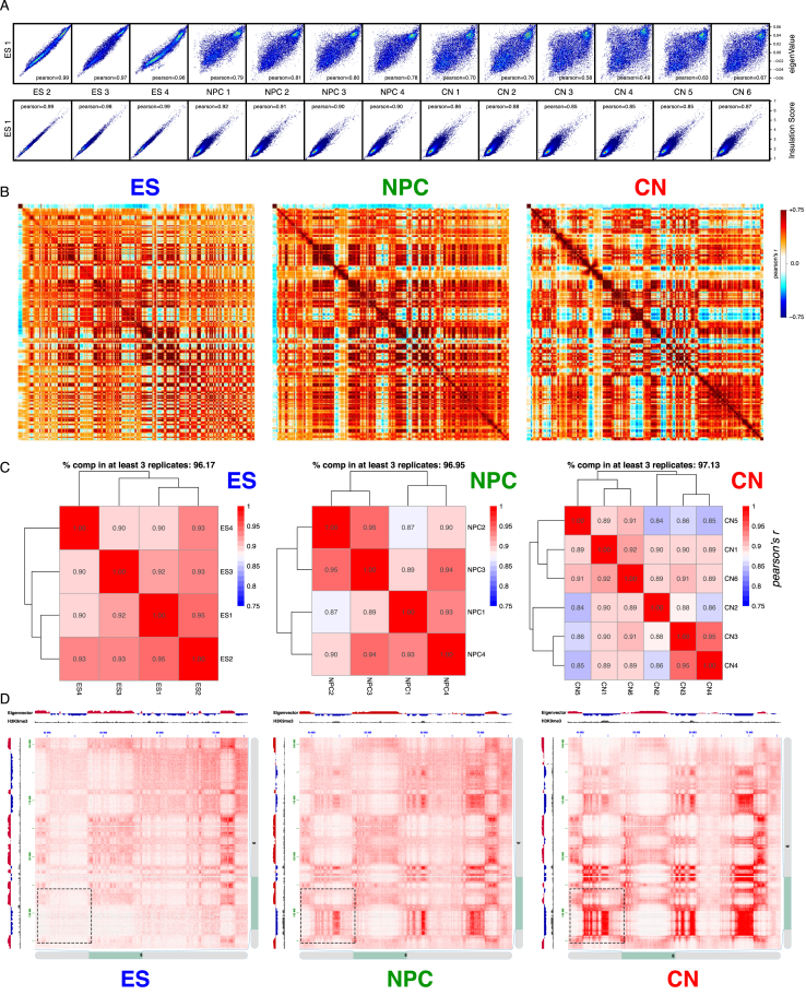
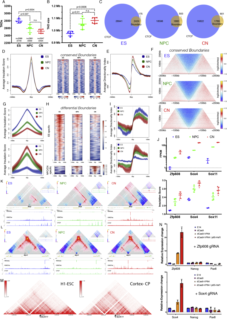
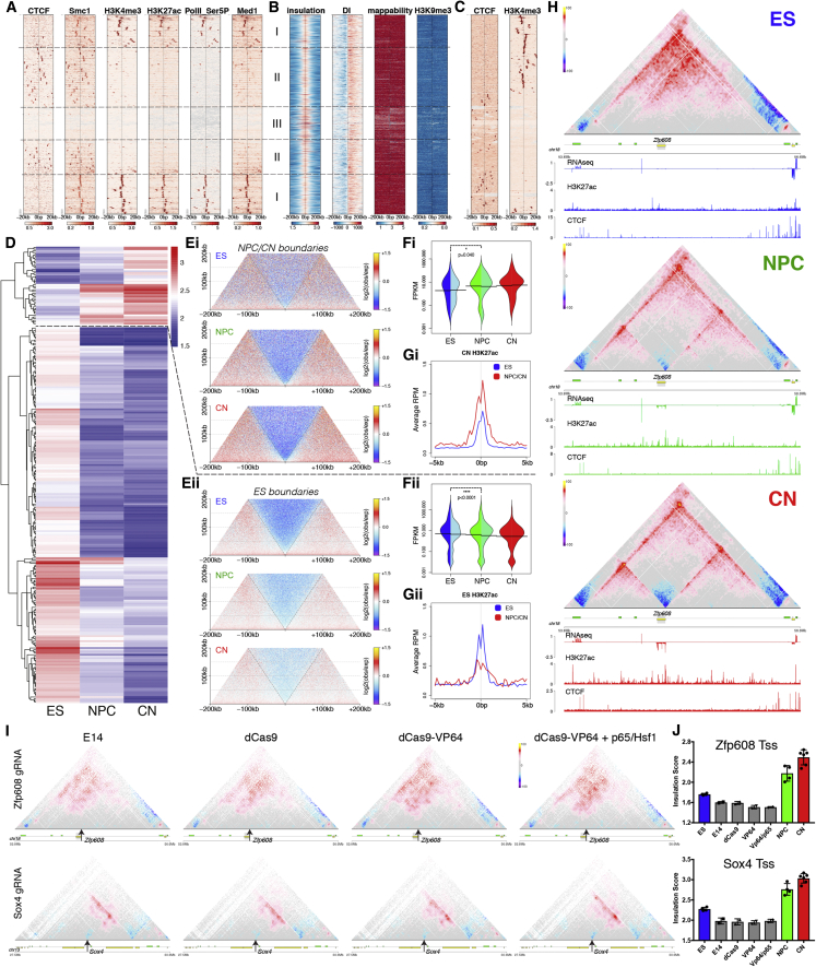
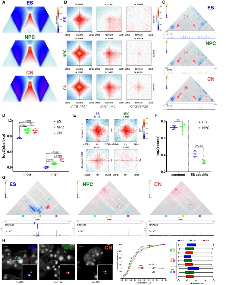
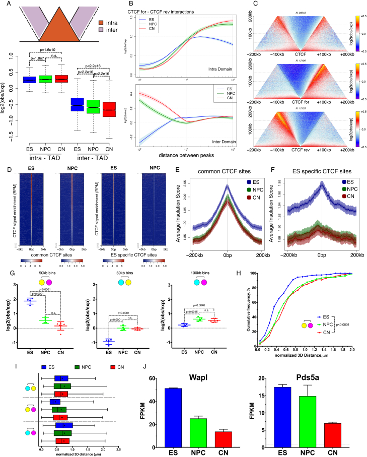
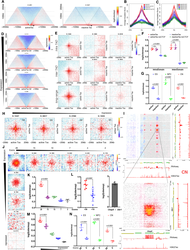
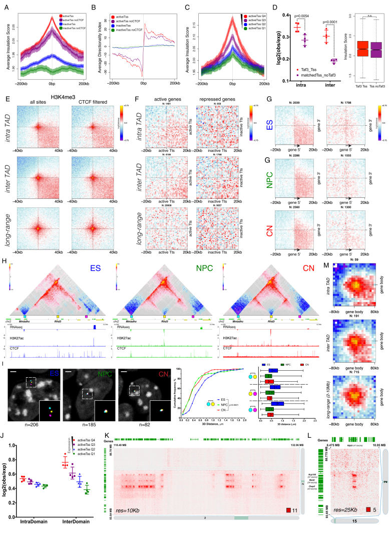
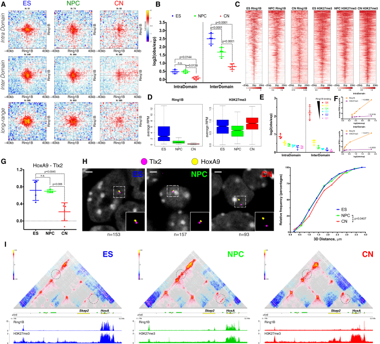
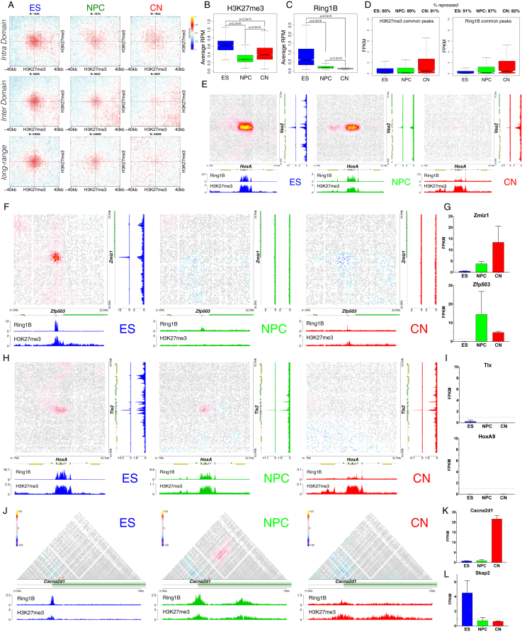
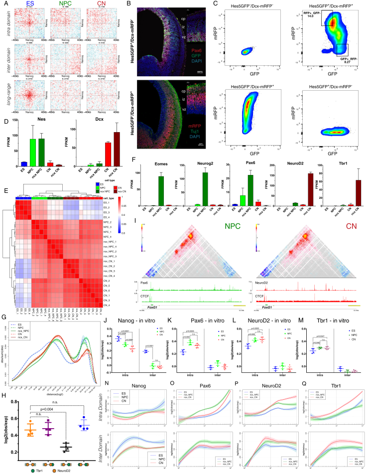
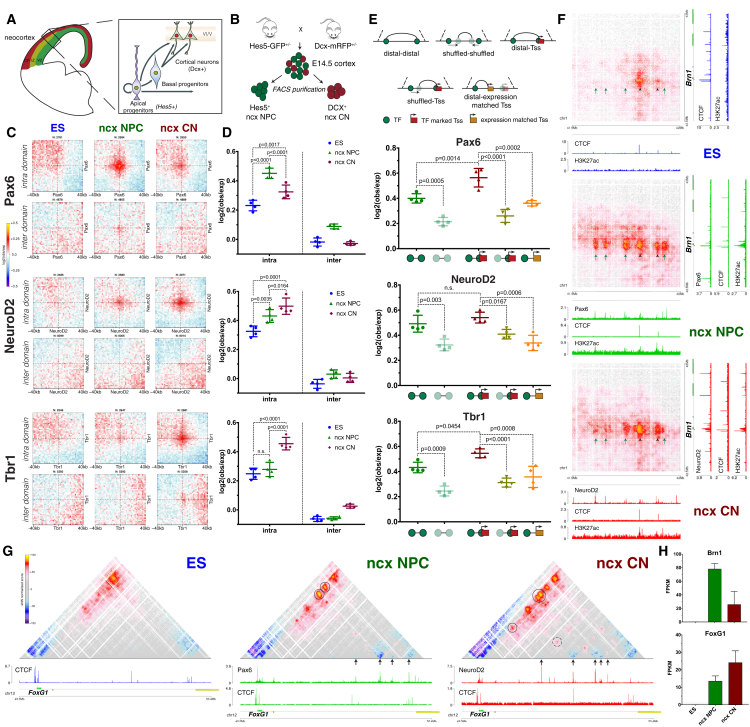
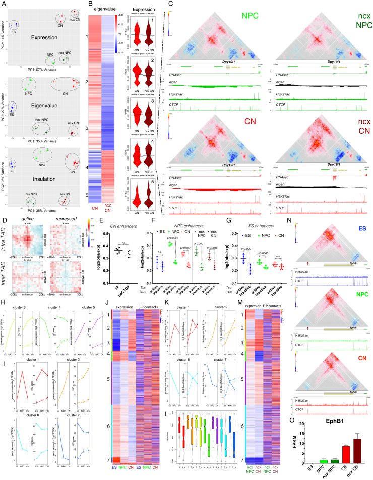
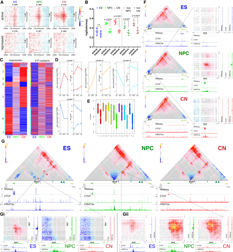
Chromosome conformation capture technologies have revealed important insights into genome folding. Yet, how spatial genome architecture is related to gene expression and cell fate remains unclear. We comprehensively mapped 3D chromatin organization during mouse neural differentiation in vitro and in vivo, generating the highest-resolution Hi-C maps available to date. We found that transcription is correlated with chromatin insulation and long-range interactions, but dCas9-mediated activation is insufficient for creating TAD boundaries de novo. Additionally, we discovered long-range contacts between gene bodies of exon-rich, active genes in all cell types. During neural differentiation, contacts between active TADs become less pronounced while inactive TADs interact more strongly. An extensive Polycomb network in stem cells is disrupted, while dynamic interactions between neural transcription factors appear in vivo. Finally, cell type-specific enhancer-promoter contacts are established concomitant to gene expression. This work shows that multiple factors influence the dynamics of chromatin interactions in development.

Keywords: 3D genome architecture; Hi-C; Polycomb; cortical development; enhancers; neural differentiation; transcription; transcription factors.

Graphical abstract

Figure S1

Ultra-Deep Hi-C during Mouse Neural Differentiation, Related to Figure 1 (A) Representative immunofluorescence images for the three cell lines used during this study. Neural differentiation is performed as described (Gaspard et al., 2008) and NPC and CN cells were obtained 12+2 or 12+9 days after changing to DDM media respectively. (B) FACS purification to select GFP⁺ population, which are also in the G₀G₁⁺ phase of the cell cycle based on DNA content. (C) Expression pattern of several markers for pluripotency, neural progenitors, differentiation or cortical neuronal subtypes. Data are represented as the mean ± SD based on two biological replicate RNaseq experiments. (D) Pearson’s correlation between two biological HiC replicates (ES1 and ES3), as a function of the genomic distance between interacting regions. (E) Pairwise Pearson’s correlation between Hi-C samples generated using the in vitro neuronal differentiation system (at 50Kb resolution and considering only contacts separated by at least 100Kb and not more than 2.6Mb). Note that the major separation occurs between cell types and also that ESs which were not sorted based on cell cycle phase (“ES_noCellCycle”) cluster separately. (F) HiC resolution achieved in this study, calculated exactly as described (Rao et al., 2014). The highest resolution Hi-C available so far – in human GM12878 cells (Rao et al., 2014) is shown as comparison. (G) Log-log contact probability as a function of the genomic distance. The exponent γ represents the mean slope ± SD of the best-fit line between 100Kb and 2Mb, multiplied by −1. (H) Contact probability as a function of the genomic distance in logarithmic bins (without dividing by bin size). Lines represent the mean values from biological replicates where available; semi-transparent ribbons show SEM. Note that while sorting itself does not have a major consequences on the contact distribution profile, samples with more cells in G₂/M are characterized by a higher proportion of close-range cis contacts. (I) Enrichment for either ChIP-seq signal or replication timing (Hiratani et al., 2010)/ Lamin B1 DamID (Peric-Hupkes et al., 2010) where available, in the two compartments. (J) Number of compartment transitions as determined using the cis-Eigenvector 1 calculated at 100Kb resolution. Shown is also the ratio of common compartment borders that are also changed between ESs and CNs compared to ESs to NPCs (±100kb). (K) Expression of the Lamin B receptor (Lbr) and Lamin B1 during neural differentiation. (L) Contact enrichment represented as the log ratio between observed and expected contacts overlapping with the indicated domain type as a function of the genomic distances. Data were smoothed using loess regression. Lines represent the mean values from biological replicates; semi-transparent ribbons show SEM.

Figure 1

Global Reorganization of 3D Genome Architecture during Neural Development (A) Schematic representation of the in vitro system. (B) Observed contact matrices for chr3 at 250-kb resolution and the first eigenvector at 100-kb resolution. Scale bar is adjusted to account for the total coverage on chr3 in each cell type. (C) Contact probability in logarithmic bins. Lines: mean values from biological replicates; semi-transparent ribbons: SEM. (D) Number of borders between adjacent TADs of different type normalized by the total number of TAD boundaries. Error bars represent SD. Shown also is the percentage of common compartment borders that are also changed between ESs and CNs compared to between ESs and NPCs (± 100 kb). (E) Contact enrichment between domains from the same (“A” versus “A” or “B” versus “B”) and different (“A” versus “B”) type. Data are represented as a scatter dot plot showing the mean ± SD. Statistical significance is calculated using two-way ANOVA with Tukey’s test. (F) Average contact enrichment between pairs of 100-kb loci arranged by their eigenvalue (shown on top). (G) Spearman’s correlation between the eigenvector value and ChIP-seq signal enrichment in 100-kb bins. (H) Hi-C contact map between two B-type regions. Each point represents a contact, color-coded according to the density of the observed contacts around it, normalized by the density of the expected contacts (STAR Methods). See also Figure S1 and S2 and Tables S1 and S2.

Figure S2

Hi-C Compartments and Reproducibility across Replicates, Related to Figure 1 (A) Example scatterplots showing the correlations between eigenvalues or insulation score between ES1 and the rest of the samples. (B) Pearson correlation Hi-C matrices for chr3 based on pooled data at 100kb resolution. (C) Classification of domains into A and B type is robust across replicates. Shown is the correlation when domains are assigned to the A- or the B- compartment in individual replicates and percentage of domains with identical classification in at least 3 replicates. (D) Hi-C contact map at 50kb resolution generated using Juicebox (Rao et al., 2014) showing increased interactions within the B-compartment during differentiation. Shown is also the eigenvector and the H3K9me3 ChIP-seq from the corresponding cell type. Region shown in Figure 1H is highlighted with a dashed square.

Figure S3

Cell-Type Specific TAD Boundaries Can Be CTCF-Independent and Are Frequently Correlated with Active Promoters, Related to Figure 2 (A) The number of TADs identified in this study. Data are represented as a scatter dot plot showing the mean ± SD. Shown is also the number of TAD boundaries identified in at least 3 biological replicates. (B) Average TAD size in the three cell types. Data are represented as a scatter dot plot showing the mean ± SD. (C) Overlap between TAD boundaries and CTCF sites in a 20Kb window. Multiple sites (boundaries or CTCF binding sites) within this window were counted only once. Note the gradual increase of CTCF^- TAD boundaries during differentiation. (D) Average insulation score and heatmaps in a 1Mb region around conserved TAD boundaries. Lines show mean values, while dark and light shaded ribbons represent SD and 95%CI respectively. (E) Average directionality index (DI) in a 1Mb region centered on conserved TAD boundaries. Lines show mean values, while dark and light shaded ribbons represent SD and 95%CI respectively. Note the gradual increase in insulation with differentiation. (F) Aggregate HiC maps centered on the conserved TAD boundaries. Data are presented as the log ratio of observed and expected contacts in 500bp bins. (G) Average insulation score a 200Kb region centered on either ES, or NPC/CN specific TAD boundaries. Lines show mean values, while dark and light shaded ribbons represent SD and 95%CI respectively. (H) Heatmaps representing the insulation score in a 200Kb region centered on either ES, or NPC/CN specific TAD boundaries. (I) Average DI a 200Kb region centered on either ES, or NPC/CN specific TAD boundaries. Lines show mean values, while dark and light shaded ribbons represent SD and 95%CI respectively. (J) Expression of Zfp608, Sox4 and Sox11 represented as the mean ± SD on a log10 scale. Also shown is the maximum insulation score at the Tss ± 10kb. (K) Hi-C maps in ∼3Mb region around Sox4 gene (shaded). Shown are also RNaseq, H3K27ac and CTCF ChIP0seq tracks in each cell type. Scale bars represent RPM. Insets show a magnified view of the region around Sox4 promoter (arrow). (L) HiC maps in ∼3Mb region around Sox11 gene (shaded). Shown are also transcriptional output (RNaseq), H3K27ac and CTCF ChIP-seq tracks in each cell type. Scale bars represent RPM. Insets show a magnified view of the region around Sox11 promoter. (M) Hi-C maps around the human SOX11 locus obtained through the 3D Genome Browser at http://www.3dgenome.org/ZMcSZ/ using publically available data (Dixon et al., 2015, Won et al., 2016). (N) qPCR showing the relative expression of the targeted gene locus upon CRISPR-dCas9 activation. E14 represents ESs infected only with the guideRNA, dCas9/dCas9-VP64/dCas9-VP64+p65-Hsf1 are stable cell lines expressing the indicated form of dCas9, infected with the indicated guide RNA. The values of each replicate (N = 2) is shown together with the mean ± SD. The expression of ES (Nanog) or NPC (Pax6) marker gene is shown as a comparison.

Figure 2

Transcription Is Correlated with but Not Sufficient to Cause Insulation at TAD Boundaries (A–C) Signal enrichment centered on TAD boundaries in ES (A and B) or CN (C) cells. Rows were ordered using hierarchical clustering. The three main classes (Tss: I, CTCF: II and repeats: III) are highlighted. (D) Hierarchical clustering of differential TAD boundaries based on the insulation score. We denote the two major clusters as ES-specific boundaries: n = 259, and neural-specific boundaries: n = 54. (E) Aggregate Hi-C maps centered on either neural-specific (Ei) or ES-specific (Eii) TAD boundaries. (F) Beanplots showing expression of genes in close proximity (< 10 kb) of a differential boundary. Each half of the bean represents a separate RNA-seq replicate. Lines show the mean value per replicate. p value is calculated using Wilcoxon rank-sum test. (G) Average enrichment of H3K27ac in CNs (Gi) or ESs (Gii) at differential TAD boundaries. (H) Example of a novel neural boundary at the Zfp608 locus. (I) Hi-C maps at the Zfp608 and Sox4 loci upon CRISPR-dCas9 gene activation. (J) Average insulation score at the Zfp608 or Sox4 Tss ± 5 kb. Data are presented as mean ± SD. The values based on the high-resolution Hi-C samples (ES, NPC, and CN) are shown as comparison. In all panels, genes transcribed in the forward direction are represented by green rectangles and genes in the reverse orientation are represented by yellow. See also Figure S3 and Table S2.

Figure 3

Stronger Loops between Convergent CTCF Sites and Dynamic Chromatin Contacts at Cell-Type Specific CTCF Sites (A) Average TAD representation in each cell type. Note the increase in contact enrichment at the domain loop. (B) Aggregate Hi-C map around pairs of convergent CTCF binding sites in each cell type. (C) Example of a Hi-C map at a conserved region. Note the increase of contact enrichment between CTCF sites (between domain boundaries: circle, inter-TAD: dashed circle). (D) Scatter dot plot showing the mean ± SD contact enrichment between convergent CTCF sites. Statistical significance is calculated using two-way ANOVA with Tukey’s test. (E and F) Aggregated contacts and quantification around intra-TAD pairs of convergent CTCF binding sites either present in both ESs and NPCs (“common CTCF”) or ES specific. Data are represented as a scatter dot plot showing the mean ± SD. Statistical significance is calculated using two-way ANOVA with Tukey’s test. (G) Hi-C contact maps at the Zfp42 locus. Regions examined by FISH are indicated with colored squares. (H) Representative 3D-DNA FISH images (z-slice) and quantification for the regions shown in (G). In all panels, n refers to the number of pairs examined. See also Figure S4 and Table S4.

Figure S4

Dynamic CTCF Contacts Contribute to Cell-Type Specific 3D Genome Architecture, Related to Figure 3 (A) Contact enrichment intra- and inter-TAD during differentiation (STAR Methods). Data represented as a boxplot based on the intra- and inter- values per TAD. Statistics are calculated using the unpaired Wilcoxon test. (B) Contact enrichment between pairs of convergent CTCF sites represented as the log ratio between observed and expected contacts as a function of the genomic distances. Data were smoothed using loess regression. Lines represent the mean values from biological replicates; semi-transparent ribbons show SEM. (C) Aggregate Hi-C maps in ESs centered on the top 30000 CTCF binding sites based on ChIP enrichment in ESs (separated based on the orientation of the CTCF motif). (D) Heatmaps showing CTCF ChIP-seq signal enrichment around either common sites (present in ESs and NPCs), or ES-specific sites. (E and F) Average insulation score centered around either conserved or ES specific CTCF sites. Lines show mean values, while dark and light shaded ribbons represent SD and 95%CI respectively. (G) Quantification of the contact enrichment between the regions shown in Figure 3G between either 50kb or 100kb bins centered on the middle of the FISH probe region. Data are presented as a scatter dot plot showing the mean ± SD. Statistical significance is calculated using one-way ANOVA with Tukey’s correction. (H) Distribution of the normalized 3D FISH distances between the regions showed in Figure 3G. (STAR Methods). (I) Quantification of the normalized FISH distances between the regions showed in Figure 3G. (J) Expression of the cohesin unloading complexes Wapl and Pds5a decreases during neural differentiation. Shown is the mean ± SD based on the RNaseq data.

Figure 4

Long-Range Interactions between Active Promoters and Gene Bodies with Many Exons (A) Aggregate Hi-C maps in NPCs centered on either active or repressed gene promoters with no CTCF binding site within ± 5 kb. (B) Average insulation score centered on gene promoters in NPCs. Lines show mean values; dark and light shaded ribbons represent SD and 95% confidence interval, respectively. (C and D) Average insulation score (C) and aggregate Hi-C maps (D) centered on active gene promoters in NPCs separated into quartiles based on expression. (E) Aggregate Hi-C contact maps around pairs of gene promoters in NPCs with no CTCF binding site within ± 5 kb. (F and G) Quantification of the contact strength between pairs of either active or repressed Tss (F) or between inter-TAD pairs of either active or repressed Tss (G). Data are represented as a scatter dot plot showing the mean ± SD. Statistical significance is calculated using two-way ANOVA with Tukey’s test. (H) Aggregate Hi-C contact maps around pairs of active gene promoters in NPCs separated into quartiles based on expression. Shown are long-range (2- to 10-Mb) inter-TAD interactions. (I) Example of clusters of long-range loops between gene bodies in CNs. Also shown is a zoomed-in interaction between the Ckap5 and Ubr1 genes and quantification of the contact enrichment. Genes transcribed in the forward direction are represented by green rectangles and genes in the reverse orientation are represented by yellow. (J) Aggregate Hi-C maps between long-range (10- to 50-Mb) pairs of genes (central bin represents the middle of the gene) separated in quantiles based on either number of exons (shown is the average number of exons in a quantile) or gene expression. Shown are 160 × 160 kb windows with a bin size of 8 kb. (K–N) Quantification of the contact enrichment between genes (25-kb bins around the center of the gene) by the average number of exons (K), by the number of exons in genes with comparable length (L), by average expression (M), and in different cell types (N). Data are represented as a scatter dot plot showing the mean ± SD. Statistical significance is calculated using two-way ANOVA with Tukey’s test. In all panels, n refers to the number of intervals or pairs examined. See also Figure S5.

Figure S5

Transcription-Associated Contacts and Local Chromatin Insulation around Gene Promoters, Related to Figure 4 (A) Average insulation score centered on gene promoters in ESs. Lines show mean values, while dark and light shaded ribbons represent SD and 95%CI respectively. (B) Average DI centered on different types of gene promoters in NPCs. (C) Average insulation score centered on active gene promoters in ESs separated into quartiles based on expression values in ESs. (D) Quantification of the contact enrichment and insulation at Tss which are bound by Taf3 or expression matched Tss which are not bound Taf3 in ESs. Statistics are calculated using two-way Anova with Sidak’s correction (contacts) or the Wilcoxon’s unpaired test (insulation). (E) Aggregate Hi-C maps in NPCs between pairs of either all H3K4me3 sites or filtered for the presence of CTCF binding site within ± 5Kb. (F) Aggregate Hi-C contact maps around pairs of gene transcription termination sites separated into active or inactive based on expression. (G) Aggregate Hi-C maps showing the interactions between matched gene promoters and transcription termination sites. Only genes longer than 50Kb and not spanning a TAD border are examined. (H) Hi-C contact maps showing ∼2.5Mb region around the Rnd3 gene. Regions examined by FISH are indicated with colored squares. (I) Representative 3D- DNA FISH images (z-slices) and quantifications showing the decrease in distance between the regions shown in (H). (J) Quantification of the contact enrichment between pairs of active gene promoters separated into quartiles based on expression. Data are represented as a scatter dot plot showing the mean ± SD. (K and L) Cluster of long-range chromatin loops either in cis (K) or in trans (L), visualized using Juicebox (Rao et al., 2014). (M) Aggregate Hi-C maps between pairs of genes in the top expression and number of exons quantile based on Figure 4J.

Figure 5

Contacts between Polycomb-Bound Regions Are Disrupted during Neural Differentiation (A and B) Aggregate Hi-C maps and quantification between pairs of regions bound by Ring1B in all three cell types. n refers to the number of pairs examined. Data are represented as a scatter dot plot showing the mean ± SD. Statistical significance is calculated using two-way ANOVA with Tukey’s test. (C and D) Heat maps and quantification showing the ChIP-seq signal enrichment centered on common Ring1B sites. Note the decrease in Ring1B binding, with no accompanying change in H3K27me3. (E) Quantification of the contact strength between pairs of the top 3,000 Ring1B binding sites in ESs divided into 6 quantiles based on Ring1B enrichment. (F) Plots of the average contact enrichment versus the average ChIP enrichment in ESs for either Ring1B or H3K27me3 in each quantile. Shown is also the Pearson correlation coefficient. (G) Quantification of the contact strength between a long-range Polycomb-associated contact (Tlx2 and HoxA9) based on Hi-C data. (H) Representative 3D-DNA FISH images (z-slice) and quantification showing the increase in distance between Tlx2 and HoxA9 during differentiation. Statistics are calculated using the Kolmogoroc-Smirnov test. (I) Hi-C contact maps at the HoxA cluster. NPC-specific contact between Skap2 and the HoxA cluster or an upstream Ring1B binding site are highlighted with a dashed circle. See also Figure S6 and Table S4.

Figure S6

Dynamic Long-Range Contacts between Polycomb-Bound Regions Are Disrupted during Differentiation, Related to Figure 5 (A) Aggregate HiC maps between pairs of regions bound by H3K27me3 in all three cell types. (B and C) Quantification of the average enrichment of either Ring1B or H3K27me3 in each cell type on common H3K27me3 sites. Statistics are calculated using Wilcoxon’s unpaired test. (D) Expression (mean FPKM) of genes within 10Kb of either common H3K27me3, or Ring1B binding sites. The percentage of repressed or weakly expressed genes (FPKM ≤ 5) is also indicated. (E) HiC contact maps showing long-range interaction between the HoxA cluster and Vax2. (F) HiC contact maps showing long-range interaction between the Zfp503 and Zmiz1 promoter. (G) Expression of the Zmiz1 and Zfp503 genes, represented as the mean ± SD. (H) HiC contact maps showing long-range interaction between the HoxA cluster and Tlx2. Shown are also the Ring1B and H3K27me3 ChIP-seq tracks in each cell type. (I) Expression of the Tlx2 and Hoxa9 genes, represented as the mean FPKM value from two replicates. (J) HiC contact maps showing ∼150Kb region around Cacna2d1 promoter. Note the appearance of NPC-specific Ring1B/H3K27me3 site inside Cacna2d1 gene body, which coincides with an interaction between this region and the Cacna2d1 promoter. (K and L) Expression of the Cacna2d1 or Skap2.

Figure S7

In Vivo Hi-C Reveals a Role for Neuronal Transcription Factors in Organizing Chromatin Interactions, Related to Figure 6 (A) Aggregate Hi-C maps between pairs of regions bound by Nanog in ESs. (B) Coronal section from E14.5 telencephalon (from Hes5GFP⁺/Dcx-mRFP^- or Hes5GFP^-/Dcx-mRFP⁺ littermates) showing the overlap between the apical progenitor marker Pax6 and GFP, or between mRFP and the neuronal marker Tuj1. (C) FACS approach to purify GFP⁺/RFP^- (referred to as “ncx NPC” henceafter) and GFP^-/RFP⁺ (“ncx CN”) populations from the same embryonic brains. (D) Expression of a neural progenitor (Nes) or neuronal marker (Dcx) either in vivo or in vitro. Data are represented as the mean ± SD from two biological replicates. (E) Pairwise Pearson’s correlation between Hi-C samples (at 50Kb resolution and considering only contacts separated by at least 100Kb and not more than 2.6Mb). Note that the major separation occurs between cell types. (F) Expression of a several markers highlighting some of the differences between the in vivo and the in vitro system. Data are represented as the mean ± SD. (G) Contact probability in logarithmic bins. Lines - mean values from biological replicates; semi-transparent ribbons - SEM. (H) Quantification of the contact enrichment in ncx_CN between distal, intra-TAD pairs of regions bound by the indicated combination of transcription factors. Data are represented as a scatter dot plot showing the mean ± SD. (I) Hi-C contact maps showing the same region as in Figure 6G but using the in vitro generated NPCs and CNs. (J–M) Quantification of the contact strength between pairs of Nanog (J), Pax6 (K), NeuroD2 (L) and Tbr1 (M) bound sites using the in vitro differentiation system. Data are represented as a scatter dot plot showing the mean ± SD. (N–Q) Contact enrichment represented between pairs of Nanog (N), Pax6 (O), NeuroD2 (P) and Tbr1 (Q) represented as the log ratio between observed and expected contacts as a function of the genomic distances. Data were smoothed using loess regression. Lines represent the mean values from biological replicates; semi-transparent ribbons show SEM.

Figure 6

Dynamic Chromatin Contacts around Neural Transcriptional Factors In Vivo (A) Schematic representation of the embryonic neocortex at E14.5. The three major cell types are shown. CP: cortical plate, IZ: intermediate zone, VZ: ventricular zone. (B) Schematic representation of the fluorescence-activated-cell-sorting (FACS)-based approach to purify NPCs or CNs from the neocortex in vivo. (C and D) Aggregate Hi-C maps and quantifications between pairs of transcription-factor (Pax6, NeuroD2, and Tbr1)- bound sites. Data are presented as a scatter dot plot showing the mean ± SD. Statistical significance is calculated using two-way ANOVA with Tukey’s test. (E) Schematic representation of the pairs of loci queried and quantification of the contact enrichment in the either ncx NPC (for Pax6) or ncx CN (NeuroD2 and Tbr1). Data are represented as a scatter dot plot showing the mean ± SD. Statistical significance is calculated using one-way ANOVA with Tukey’s test. (F) Hi-C contact maps showing interaction between Brn1 promoter and several Pax6 binding sites (green arrows) and contacts between CTCF sites (black arrowheads). (G) Example of a dynamic chromatin loops established between TF-bound sites (arrows) at the FoxG1 locus. Interactions between a distal TF-bound site and FoxG1 are highlighted with a circle and cell-type specific interaction between two distal sites is shown with a dashed circle. (H) Brn1 and FoxG1 expression represented as the mean ± SD of two biological replicate RNA-seq experiments. In all panels, n refers to the number of pairs examined. See also Figures S7 and S8.

Figure S8

Differences between In Vivo and In Vitro Hi-C and Dynamic E-P Interactions, Related to Figures 6 and 7 (A) Principal component analysis based on gene expression, average eigenvalue in 100kb bins or average insulation score in 10kb bins. (B) K-means clustering of the eigenvalue at regions which change compartment between in vitro and in vivo. Shown is also a beanplot representing the RNA expression of genes in a cluster. Each half of the bean represents a separate RNaseq replicate. Lines show the mean value per replicate. (C) Example of a locus, which switches between B and A compartments and becomes highly expressed only in the in vivo cortical neurons. (D) Aggregate Hi-C maps between pairs of enhancers and either active or inactive promoters identified in CNs divided into two groups: intra domain (pairs lie inside TADs and are separated by more than 50Kb and less than 2Mb) and inter domain (pairs lie between TADs but are separated by the same distance as before). Genes were oriented according the direction of transcription. (E) Quantification of the contact strength of intraTAD pairs between CN enhancers (all or filtered for the presence of a CTCF binding site within ± 5Kb) and active CN promoters. (F) Quantification of the contact strength of intraTAD pairs between NPC enhancers and either NPC active or repressed promoters. Data are represented as a scatter dot plot showing the mean ± SD. Statistical significance is calculated using two-way ANOVA with Šídák’s multiple comparison correction. (G) As in (F) but considering pairs of ES enhancers and ES active or repressed promoters. (H) Average expression or average enhancer-promoter Hi-C score within the specified cluster (from Figure 7C). Shown are also the average Hi-C scores when enhancers were randomly shuffled within the same TAD. Error bars indicate ± SEM. (I) Same as in (H) but based on in vivo data. (J) Heatmap showing gene specificity scores (STAR Methods) based on either gene expression or the average enhancer-promoter interactions (per gene) in vitro. Clusters are the same as in Figure 7C. (K) Average gene specificity scores based on either expression or Hi-C contacts within the specified cluster. Shown are also the average Hi-C scores when enhancers were randomly shuffled within the same TAD. Error bars indicate ± SEM. (L) Boxplots representing the Pearson’s correlation between expression and contacts-based gene specificity score within a cluster. (M) Same as in (J) but based on the in vivo data. (N) Hi-C contact maps showing ∼2.5Mb region around EphB1 promoter. The location of a putative CN specific enhancer is shown by red arrow. Note that this coincides with a conserved CTCF-binding site occupied in all three cell types. (O) EphB1 expression, represented as the mean ± SD from two biological replicates.

Figure 7

Enhancer-Promoter Contacts Are Mostly Cell-Type Specific and Are Correlated with Gene Expression (A and B) Aggregate Hi-C maps and quantification between intra-TAD pairs of enhancers and either active or inactive promoters identified in CNs. Genes were oriented according to the direction of transcription. Data are represented as a scatter dot plot showing the mean ± SD. Statistical significance is calculated using two-way ANOVA with Šídák correction. (C) Heat map showing Z scores based on either gene expression (fragments per kb of transcript per million mapped reads [FPKM]) or the average E-P interactions per gene. Genes are partitioned using k-means clustering on the RNA expression data across all cell types. (D) Average expression or average E-P Hi-C score within the specified cluster. Shown are also the average Hi-C scores when the enhancer contact anchor was randomly shuffled within the same TAD (dashed lines). Error bars indicate ± SEM. (E) Boxplots representing the Pearson correlation coefficient between expression and average E-P interactions per gene, either real or shuffled (shuffled are indicated by the “_s” prefix). (F) Hi-C contact maps showing ∼2.6-Mb region around Brn2 promoter. Insets show a magnified view of the contact between the Brn2 promoter and an NPC-specific enhancer (dashed circle). (G) Hi-C contact maps showing ∼2-Mb region at the Sox2 locus. The positions of two putative NPC-specific enhancers are indicated by green arrowheads. Insets showing the interaction between Sox2 promoter and an ES-specific enhancer (blue arrow, Gi); or Sox2 promoter and a known NPC-specific enhancer (green arrow, Gii). See also Figure S8 and Table S3.

References

1. Bantignies F., Roure V., Comet I., Leblanc B., Schuettengruber B., Bonnet J., Tixier V., Mas A., Cavalli G. Polycomb-dependent regulatory contacts between distant Hox loci in Drosophila. Cell. 2011;144:214–226. - PubMed
1. Basak O., Taylor V. Identification of self-replicating multipotent progenitors in the embryonic nervous system by high Notch activity and Hes5 expression. Eur. J. Neurosci. 2007;25:1006–1022. - PubMed
1. Bayam E., Sahin G.S., Guzelsoy G., Guner G., Kabakcioglu A., Ince-Dunn G. Genome-wide target analysis of NEUROD2 provides new insights into regulation of cortical projection neuron migration and differentiation. BMC Genomics. 2015;16:681. - PMC - PubMed
1. Bibel M., Richter J., Schrenk K., Tucker K.L., Staiger V., Korte M., Goetz M., Barde Y.-A. Differentiation of mouse embryonic stem cells into a defined neuronal lineage. Nat. Neurosci. 2004;7:1003–1009. - PubMed
1. Bonev B., Cavalli G. Organization and function of the 3D genome. Nat. Rev. Genet. 2016;17:661–678. - PubMed