Recycled iron fuels new production in the eastern equatorial Pacific Ocean

Abstract

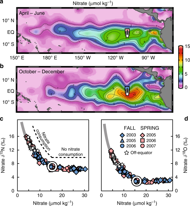
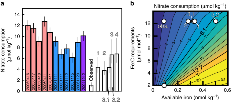
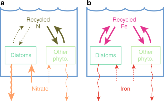
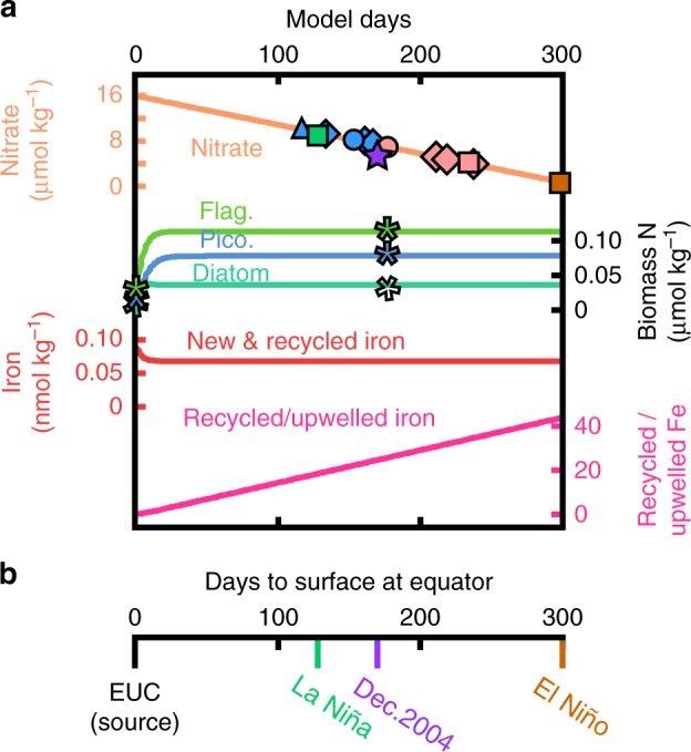
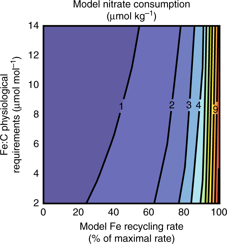
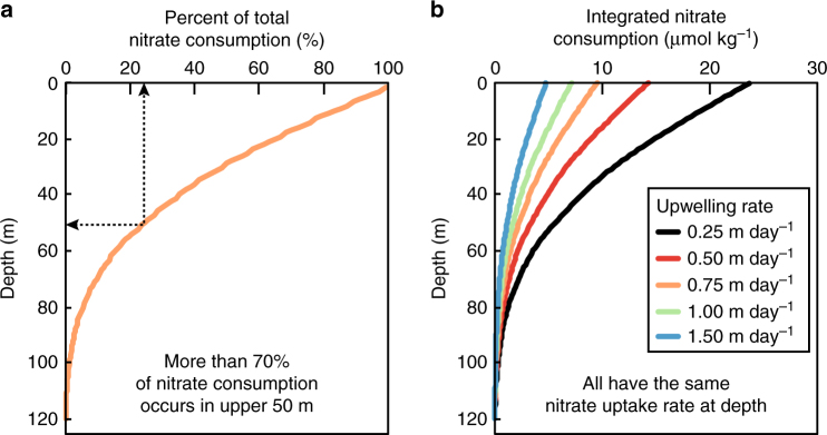
Nitrate persists in eastern equatorial Pacific surface waters because phytoplankton growth fueled by nitrate (new production) is limited by iron. Nitrate isotope measurements provide a new constraint on the controls of surface nitrate concentration in this region and allow us to quantify the degree and temporal variability of nitrate consumption. Here we show that nitrate consumption in these waters cannot be fueled solely by the external supply of iron to these waters, which occurs by upwelling and dust deposition. Rather, a substantial fraction of nitrate consumption must be supported by the recycling of iron within surface waters. Given plausible iron recycling rates, seasonal variability in nitrate concentration on and off the equator can be explained by upwelling rate, with slower upwelling allowing for more cycles of iron regeneration and uptake. The efficiency of iron recycling in the equatorial Pacific implies the evolution of ecosystem-level mechanisms for retaining iron in surface ocean settings where it limits productivity.

Fig. 1

Tropical Pacific nitrate concentration and isotopic composition. Tropical Pacific surface nitrate concentrations for a April–June and b October–December, with squares and stars indicating station locations. c, d show nitrate δ ¹⁵N and δ ¹⁸O measurements vs. nitrate concentration for the samples from these stations. Pink and blue symbols are ±1° of equator during boreal spring and fall, respectively. White stars indicate 2–4° S surface mixed layer measurements. Plotted data are from the upper 200 m of the water column. White circles in c, d indicate the averages of measurements of the Equatorial Under Current (EUC) at 110° W, and these values are used to drive the Rayleigh (closed system) model of nitrate assimilation (gray lines) (see text for more details)

Fig. 2

Observed and potential nitrate consumption. a Nitrate consumption estimates from 2003 to 2007 (colored bars) compared with potential nitrate consumption calculated for Scenarios 1–4 (open bars). Nitrate consumption estimates in a are from spring (pink), fall (blue), winter (purple), and error bars are ±1 μmol kg⁻¹ based on source water variability (sampling date at bottom; values in Tables 1 and 2). White columns represent nitrate consumption predicted based on the following scenarios. "Observed" uses iron supply and diatom Fe:C requirements that match local observations^, . Scenario 1 uses local observations, but with a doubled dust-borne iron supply and an order of magnitude higher solubility of dust-borne iron. Scenario 2 assumes all particulate iron is bioavailable. Scenarios 3.1 and 3.2 use dissolved iron concentrations from 200 m and EUC measurements 3300 km west, respectively. Scenario 4 uses the lowest reported diatom Fe:C requirement of 2 μmol mol⁻¹ . Error bars (1 standard deviation) allow for potential C:N variability of ±2 (global community value) even though phytoplankton community C:N ratio in the eastern equatorial Pacific is much smaller (±0.3). b A sensitivity analysis of potential nitrate consumption based on available iron concentrations and physiological iron requirements. White numbers in b indicate the Scenarios from a, none of which can explain the observed range in nitrate consumption of 6.1 and 12.7 μmol kg⁻¹ (bold contours)

Fig. 3

Distinct iron and nitrogen cycling pathways and their affect on nitrate consumption. Conceptual models of a nitrogen (N) and b iron (Fe) transformation pathways in the eastern equatorial Pacific, where nutrient consumption is shown by a straight arrow, nutrient regeneration by a curved arrow, and wavy arrows denote export. Arrow size denotes relative flux size, and dashed arrows are very small fluxes (see text for details). Other phyto. refers to non-diatom phytoplankton, including autotrophic flagellates and picoplankton, which primarily meet their N requirements with recycled N (see “Methods”). The preferential regeneration of iron relative to nitrogen predicts a higher export of nitrogen relative to iron

Fig. 4

Biogeochemical model of upwelled equatorial water. a The output of a numerical box model following the nutrient transformations shown in Fig. 3 shows the observed decline in nitrate and increase in phytoplankton biomass nitrogen (N) at our study site^, . Model dissolved iron concentrations (Fe) include both upwelled new and recycled iron and therefore do not drop to the lowest observed regional surface ocean values (≈0.02 nmol kg⁻¹)^, . The ratio of recycled to upwelled iron indicates the degree of iron recycling required to drive the nitrate consumption. Symbols plotted over the modeled nitrate concentration indicate surface nitrate concentration observations from the seasonal stations (orange and purple symbols, Fig. 1), from December 2004 (purple star), and for La Niña (green square) and El Niño conditions (brown square) (based on ref. ). Asterisks mark biomass N targets for model tuning at 0.1% and 100% light levels for photosynthetic flagellates (flag.), picoplankton (pico.), and diatoms. b The rate at which waters upwell from the Equatorial Under Current (EUC) and advect away from the equator affects its residence time at the equator (how long water takes to upwell to the surface). Here we represent this variable time scale based on surface nitrate concentrations for the December 2004 measurements (purple) and during La Niña and El Niño conditions. Poleward advection of these waters once they reach the surface should scale accordingly, explaining the observed changes in the spatial extent of HNLC waters

Fig. 5

Sensitivity analysis of model nitrate consumption. Modeled nitrate consumption at 200 model days as a function iron recycling rate (X-axis) and iron: carbon (Fe:C) physiological requirement (Y-axis). With no iron recycling and a Fe:C requirement of 12.3, the model predicts nearly identical nitrate consumption as the stoichiometric calculation using observed values (0.9 vs. 1.1 μmol kg⁻¹; Supplementary Table 1). Increasing model recycling and/or decreasing the Fe:C physiological requirement increases the predicted nitrate consumption. The maximal iron recycling rate considered is based on optimized model settings (see “Methods”)

Fig. 6

Simple models of nitrate consumption at the equator. Nitrate consumption increases as equatorial waters upwell towards the surface, and the degree of consumption is related to upwelling stength. Here we plot the nitrate consumption a as a percentage of the initial nitrate concentration and b in terms of nitrate concentration with varying upwelling rates. The integrated percentage of nitrate consumption in a is based on observed nitrate uptake rate with depth and total nitrate consumption (Table 1) at 0° N, 110° W from December 2004. Note that most nitrate consumption occurs in the upper 50 m, suggesting that light limitation can only play a minor role in modifying elemental requirements (e.g., lower C:N at lower light levels). The same nitrate uptake rates were used to calculate the integrated nitrate consumption in b for a variety of upwelling rates, and we found that increasing upwelling rate decreases the integrated nitrate consumption in the water upwelling at the equator (see "Methods"). The same source water depth and iron recycling rate are assumed in all calculations

References

-
- Dugdale RC, Goering JJ. Uptake of new and regenerated forms of nitrogen in primary production. Limnol. Oceanogr. 1967;12:196–206. doi: 10.4319/lo.1967.12.2.0196. - DOI
- Martin, J. H. Glacial-interglacial CO2 change: the iron hypothesis. Paleoceanography5, 1–13 (1990).
- Hutchins DA, DiTullio GR, Bruland KW. Iron and regenerated production: evidence for biological iron recycling in two environments. Limnol. Oceanogr. 1993;38:1242–1255. doi: 10.4319/lo.1993.38.6.1242. - DOI
- Landry MR, et al. Iron and grazing constraints on primary production in the central equatorial Pacific: an EqPac synthesis. Limnol. Oceanogr. 1997;42:405–418. doi: 10.4319/lo.1997.42.3.0405. - DOI
Publication types
MeSH terms
Substances
LinkOut - more resources
Full Text Sources
Other Literature Sources