Impact of climate change on New York City's coastal flood hazard: Increasing flood heights from the preindustrial to 2300 CE

Abstract

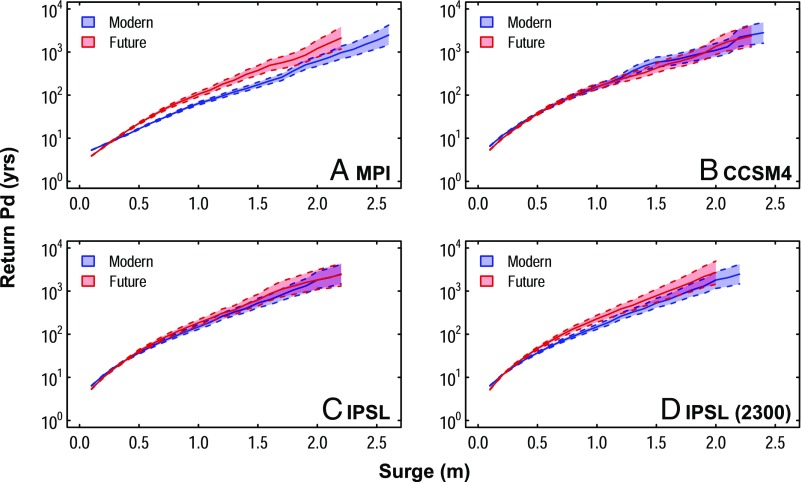
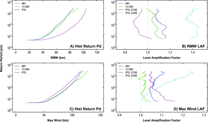
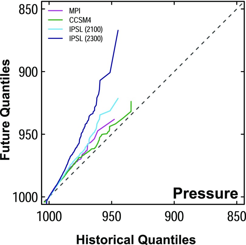
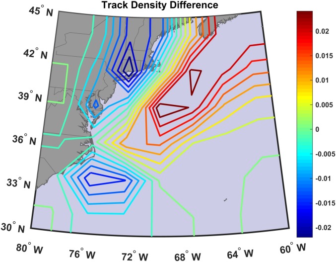
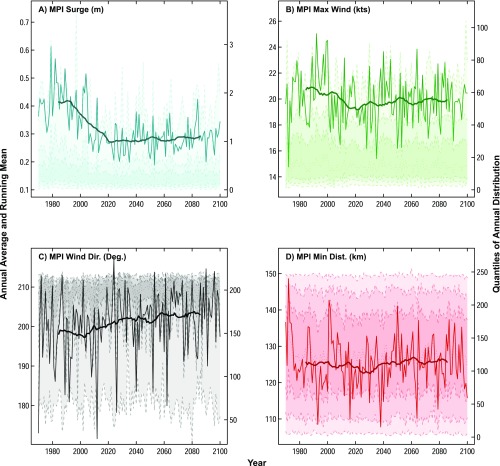
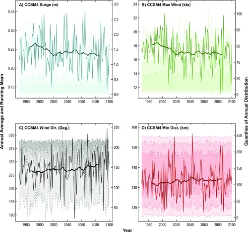
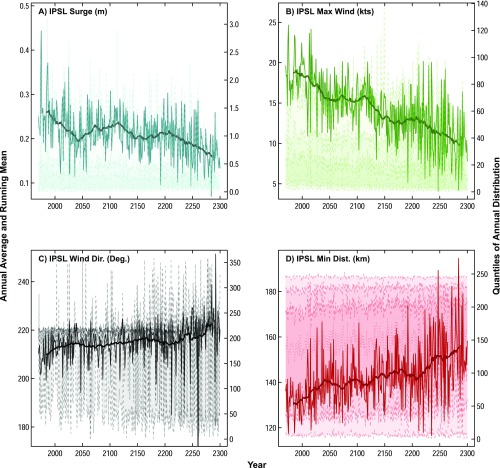
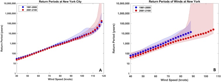
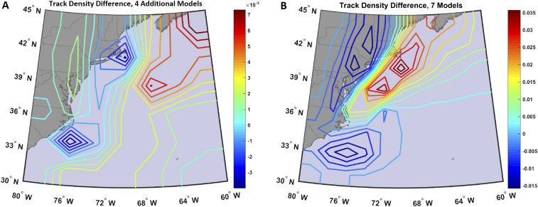
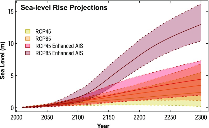
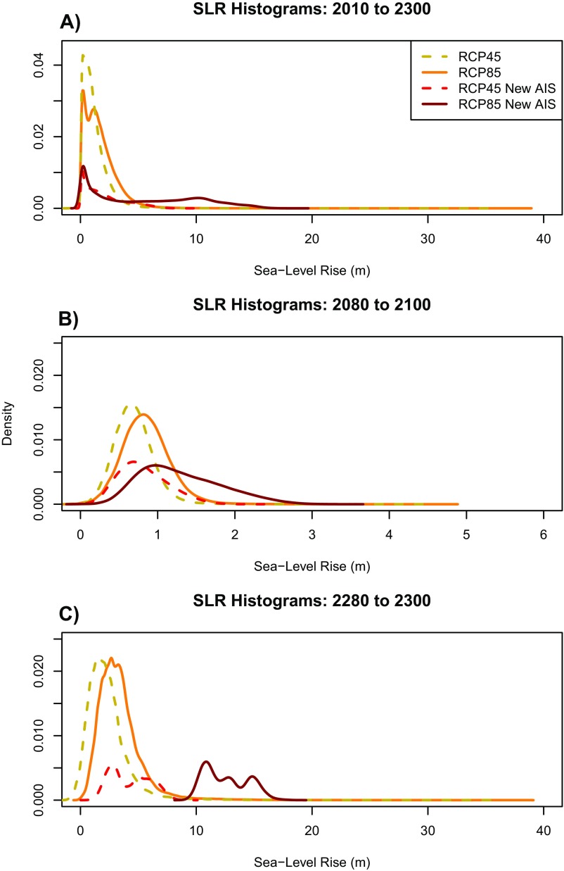
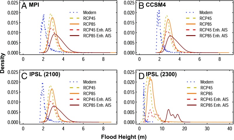
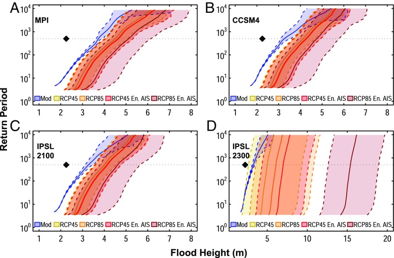
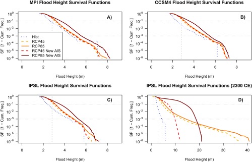
The flood hazard in New York City depends on both storm surges and rising sea levels. We combine modeled storm surges with probabilistic sea-level rise projections to assess future coastal inundation in New York City from the preindustrial era through 2300 CE. The storm surges are derived from large sets of synthetic tropical cyclones, downscaled from RCP8.5 simulations from three CMIP5 models. The sea-level rise projections account for potential partial collapse of the Antarctic ice sheet in assessing future coastal inundation. CMIP5 models indicate that there will be minimal change in storm-surge heights from 2010 to 2100 or 2300, because the predicted strengthening of the strongest storms will be compensated by storm tracks moving offshore at the latitude of New York City. However, projected sea-level rise causes overall flood heights associated with tropical cyclones in New York City in coming centuries to increase greatly compared with preindustrial or modern flood heights. For the various sea-level rise scenarios we consider, the 1-in-500-y flood event increases from 3.4 m above mean tidal level during 1970-2005 to 4.0-5.1 m above mean tidal level by 2080-2100 and ranges from 5.0-15.4 m above mean tidal level by 2280-2300. Further, we find that the return period of a 2.25-m flood has decreased from ∼500 y before 1800 to ∼25 y during 1970-2005 and further decreases to ∼5 y by 2030-2045 in 95% of our simulations. The 2.25-m flood height is permanently exceeded by 2280-2300 for scenarios that include Antarctica's potential partial collapse.

Keywords: New York City; coastal flooding; flood height; sea-level rise; tropical cyclones.

Fig. 1.

Return periods of storm-surge heights. Results are shown for the modern (blue) and future (red) periods for (A) the MPI model, (B) the CCSM4 model, (C) the IPSL model, and (D) the IPSL model where future simulations extend to 2300. The 95% credible interval of storm-surge events is shown in light blue for modern and in light red for future.

Fig. S1.

Return periods and LAFs of RMW and maximum wind. Return periods of (A) RMW values and (C) maximum wind speeds of TCs during the historic era. The LAF of the historic return periods for (B) RMW and (D) maximum wind are also shown, where LAF = (future value at given return period)/(historic value at given return period). LAF = 1 is shown by the gray dotted line.

Fig. S2.

Quantile–quantile plot of modern and future TC minimum pressure. Results are shown for MPI (magenta), CCSM4 (green), and IPSL (cyan) models from 2010 to 2100 and for the IPSL model from 2010 to 2300 (blue); pressure is considered at the time when each storm achieves its minimum distance from the Battery. The dashed line indicates the line y = x. Points that deviate from this line indicate that the two distributions being compared differ from one another.

Fig. 2.

Multimodel mean difference between future and modern synthetic TC track densities from the MPI, CCSM4, and IPSL models. Track densities are determined by the sum total of tracks crossing through each grid box over 20-y periods from 2080–2100 and 1980–2000, divided by the area of that grid box and the number of years (21). Here the grid box latitude–longitude scales are determined by the output resolution of the model in question.

Fig. S3.

Time series of TC characteristics from the MPI model. Plotted on the left y axis are the annual-mean time series from 1970 to 2100 of (A) storm-surge height (meters), (B) maximum wind speed (knots), (C) wind direction (degrees), and (D) minimum distance to The Battery (kilometers), shown by thin solid lines in the foreground; 30-y moving window averages are shown by thick solid lines on each plot. In the background of each figure, and plotted on the right y axis, are the time series of the 0.005, 0.1, 0.25, 0.5, 0.75, 0.9, and 0.995 quantiles (dashed lines). Shading highlights the 0.005–0.995 (lightest), 0.1–0.9 (medium), and 0.25–0.75 (darkest) ranges.

Fig. S4.

Time series of TC characteristics from the CCSM4 model. Plotted on the left y axis are the annual-mean time series from 1970 to 2100 of (A) storm-surge height (meters), (B) maximum wind speed (knots), (C) wind direction (degrees), and (D) minimum distance to The Battery (kilometers), shown by thin solid lines in the foreground; 30-y moving window averages are shown by thick solid lines on each plot. In the background of each figure, and plotted on the right y axis, are the time series of the 0.005, 0.1, 0.25, 0.5, 0.75, 0.9, and 0.995 quantiles (dashed lines). Shading highlights the 0.005–0.995 (lightest), 0.1–0.9 (medium), and 0.25–0.75 (darkest) ranges.

Fig. S5.

Time series of TC characteristics from the IPSL model. Plotted on the left y axis are the annual-mean time series from 1970 to 2300 of (A) storm-surge height (meters), (B) maximum wind speed (knots), (C) wind direction (degrees), and (D) minimum distance to The Battery (kilometers), shown by thin solid lines in the foreground; 30-y moving window averages are shown by thick solid lines on each plot. In the background of each figure, and plotted on the right y axis, are the time series of the 0.005, 0.1, 0.25, 0.5, 0.75, 0.9, and 0.995 quantiles (dashed lines). Shading highlights the 0.005–0.995 (lightest), 0.1–0.9 (medium), and 0.25–0.75 (darkest) ranges.

Fig. S6.

Return periods of peak wind speed at the Battery. (A) Mean return period of peak wind speed at the Battery for the MPI, CCSM4, and IPSL models during the time periods 1981–2000 and 2081–2100. (B) Mean return period of peak wind speed at The Battery for the MPI, CCSM4, IPSL, HadGEM, GFDL, MRI, and MIROC models during the time periods 1981–2000 and 2081–2100.

Fig. S7.

Changing TC track densities. (A) Multimodel mean difference between synthetic TC track densities from 2080 to 2100 and those from 1980 to 2000 for the HadGEM, GFDL, MRI, and MIROC models. (B) Multimodel mean difference between synthetic TC track densities from 2080 to 2100 and those from 1980 to 2000 for the MPI, CCSM4, IPSL, HadGEM, GFDL, MRI, and MIROC models.

Fig. 3.

Mean August and September SLP differences. Pressure differences (pascals) are between (A) 2080–2100 and 1980–2000 for all three models and (B) 2280–2300 and 1980–2000 for the IPSL model. Color bars show the range of SLP differences.

Fig. 4.

Sea-level projections from 2010 to 2300. Projections are calculated using RCP4.5 (yellow) and RCP8.5 (orange) projections (21) and for projections combining AIS contributions from ref. with the RCP4.5 (red) and RCP8.5 (dark red) projections from ref. . Lines and shaded regions represent the median and the central 95% credible interval.

Fig. S8.

Histograms of localized SLR projections for NYC. Results shown for (A) 2010–2300, (B) 2080–2100, and (C) 2280–2300 from ref. , in gold (RCP 4.5 scenario) and orange (RCP 8.5 scenario), and ref. using an AIS contribution from ref. , in red (RCP 4.5 scenario) and burgundy (RCP 8.5 scenario). Distributions represent 10,000 MC samples of projected SLR from ref. . It should be noted that SLR distributions using the AIS contribution from ref. are based on a limited number of model runs at this time and thus do not represent proper PDFs. The SLR distributions shown here are combined with future storm-surge heights to produce future flood heights.

Fig. 5.

Normalized distributions of flood heights. Distributions are for the modern (1970–2005) and future eras for flood heights calculated using the RCP4.5 and RCP8.5 SLR projections (21) and for flood heights calculated by combining enhanced AIS contributions (26) with the RCP4.5 and RCP8.5 SLR projections (21). Results are shown for future scenarios for (A) the MPI model, (B) the CCSM4 model, (C) the IPSL model, and (D) the IPSL model to 2300.

Fig. 6.

Return periods of flood heights. Results are for the modern (1970–2005) and future eras for flood heights calculated using the RCP4.5 (yellow) and RCP8.5 (orange) SLR projections (21) and for flood heights calculated by combining enhanced AIS contributions (26) with the RCP4.5 (red), and RCP8.5 (burgundy) SLR projections (21). Results are shown for future simulations for (A) the MPI model, (B) the CCSM4 model, (C) the IPSL model, and (D) the IPSL model to 2300. The gray, horizontal dotted line on each plot indicates the 500-y return period, and the black diamond on each plot indicates the 500-y flood height (2.25 m) for the preindustrial era (4); mean and 95% credible intervals of flood heights for each return period are shown by the solid line and the shaded region between dashed lines on each plot.

Fig. S9.

Survival functions of flood heights. Results are shown for the modern era (4) and future era for flood heights calculated using the RCP 4.5 (yellow) and RCP 8.5 (orange) SLR projections (21) and for flood heights calculated by combining AIS contributions from ref. with the RCP 4.5 (red) and RCP 8.5 (burgundy) SLR projections from ref. . Survival functions are shown for (A) the MPI model, (B) the CCSM4 model, (C) the IPSL model, and (D) the IPSL model where future simulations extend to 2300. Gray, horizontal dotted lines on each plot indicate the 90th- and 99.9th-percentile event frequencies; the gray, vertical dashed line on each plot indicates the flood height associated with Hurricane Sandy in 2012.

References

1. NYC Special Initiative for Rebuilding and Resiliency (2013) A stronger, more resilient New York (PlaNYC, New York)
1. Kemp AC, Horton BP. Contribution of relative sea-level rise to historical hurricane flooding in New York City. J Qua Sci. 2013;28:537–541.
1. Lin N, Emanuel KA, Oppenheimer M, Vanmarcke E. Physically based assessment of hurricane surge threat under climate change. Nat Clim Chang. 2012;2:462–467.
1. Reed AJ, et al. Increased threat of tropical cyclones and coastal flooding to New York City during the anthropogenic era. Proc Natl Acad Sci USA. 2015;112:12610–12615. - PMC - PubMed
1. Little CM, et al. Joint projections of US East Coast sea level and storm surge. Nat Clim Chang. 2015;5:1114–1120.
Publication types
LinkOut - more resources