A continuum mechanics-based musculo-mechanical model for esophageal transport

Abstract

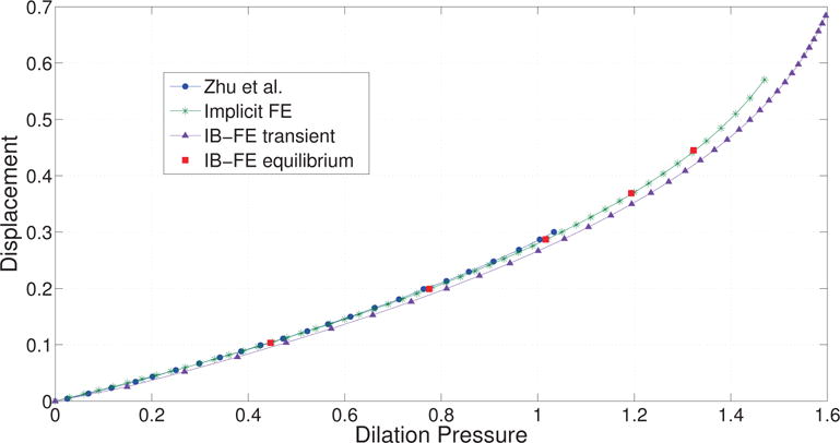
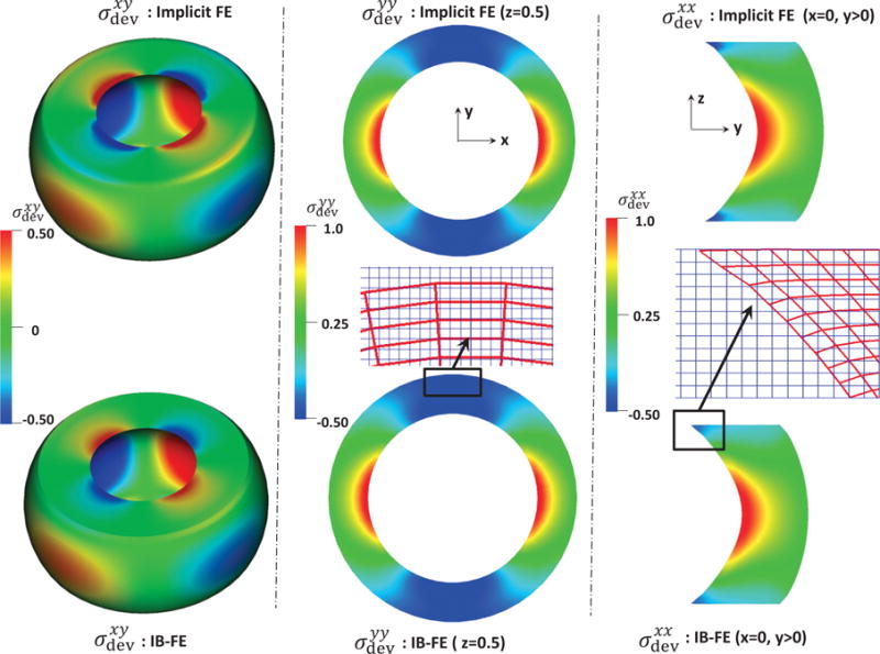
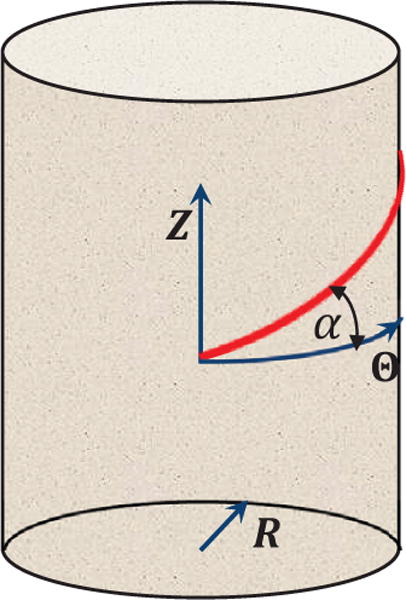
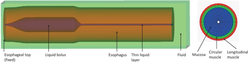
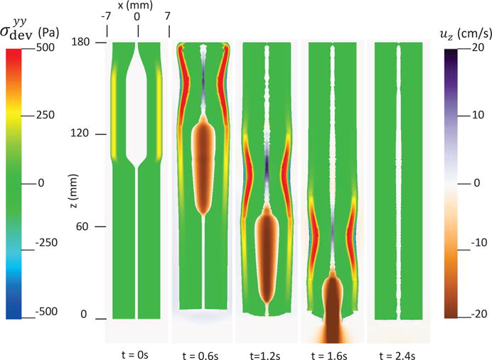
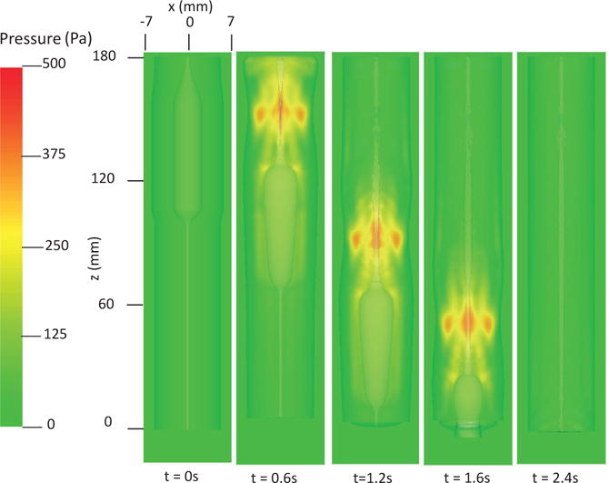
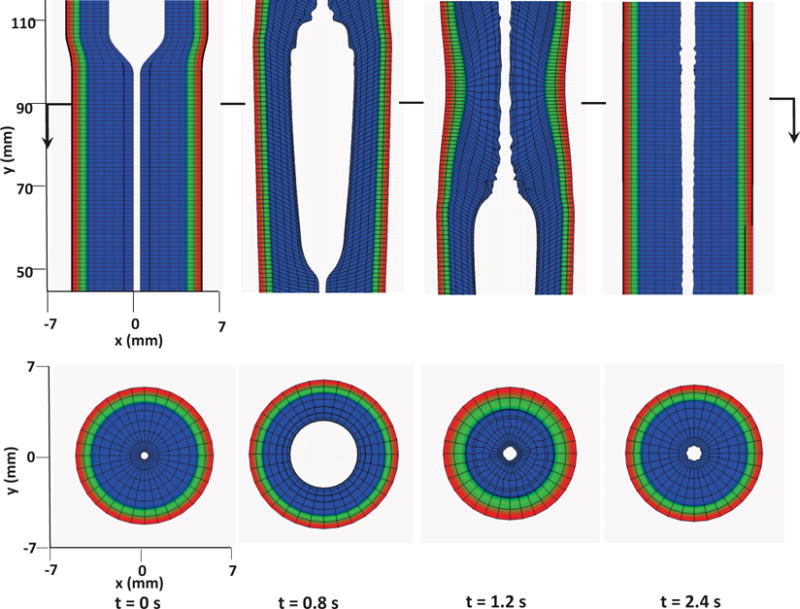
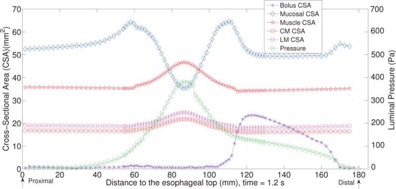
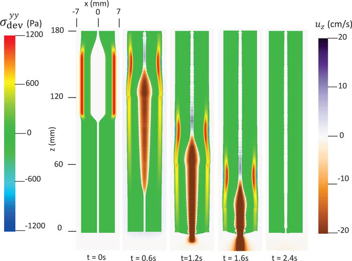
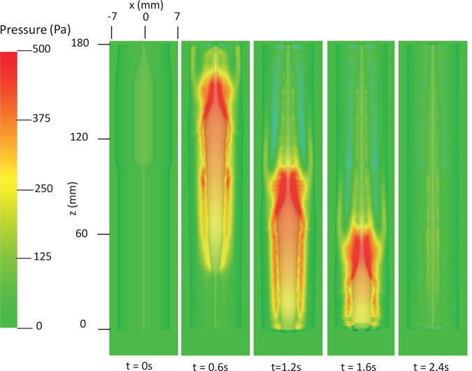
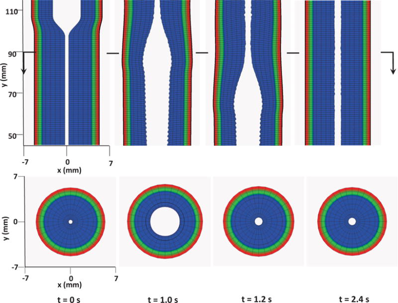
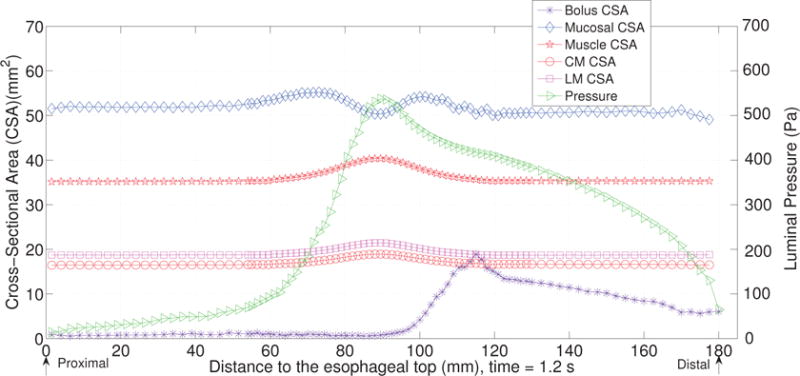
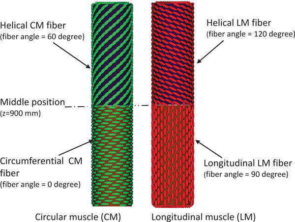
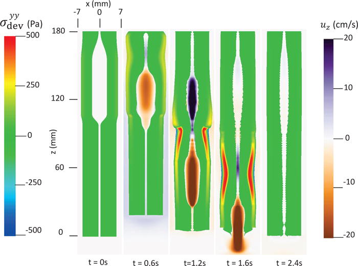
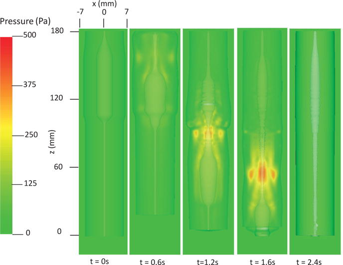
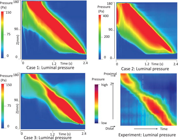
In this work, we extend our previous esophageal transport model using an immersed boundary (IB) method with discrete fiber-based structural model, to one using a continuum mechanics-based model that is approximated based on finite elements (IB-FE). To deal with the leakage of flow when the Lagrangian mesh becomes coarser than the fluid mesh, we employ adaptive interaction quadrature points to deal with Lagrangian-Eulerian interaction equations based on a previous work (Griffith and Luo [1]). In particular, we introduce a new anisotropic adaptive interaction quadrature rule. The new rule permits us to vary the interaction quadrature points not only at each time-step and element but also at different orientations per element. This helps to avoid the leakage issue without sacrificing the computational efficiency and accuracy in dealing with the interaction equations. For the material model, we extend our previous fiber-based model to a continuum-based model. We present formulations for general fiber-reinforced material models in the IB-FE framework. The new material model can handle non-linear elasticity and fiber-matrix interactions, and thus permits us to consider more realistic material behavior of biological tissues. To validate our method, we first study a case in which a three-dimensional short tube is dilated. Results on the pressure-displacement relationship and the stress distribution matches very well with those obtained from the implicit FE method. We remark that in our IB-FE case, the three-dimensional tube undergoes a very large deformation and the Lagrangian mesh-size becomes about 6 times of Eulerian mesh-size in the circumferential orientation. To validate the performance of the method in handling fiber-matrix material models, we perform a second study on dilating a long fiber-reinforced tube. Errors are small when we compare numerical solutions with analytical solutions. The technique is then applied to the problem of esophageal transport. We use two fiber-reinforced models for the esophageal tissue: a bi-linear model and an exponential model. We present three cases on esophageal transport that differ in the material model and the muscle fiber architecture. The overall transport features are consistent with those observed from the previous model. We remark that the continuum-based model can handle more realistic and complicated material behavior. This is demonstrated in our third case where a spatially varying fiber architecture is included based on experimental study. We find that this unique muscle fiber architecture could generate a so-called pressure transition zone, which is a luminal pressure pattern that is of clinical interest. This suggests an important role of muscle fiber architecture in esophageal transport.

Keywords: esophageal transport; fiber-reinforced model; fluid-structure interaction; immersed boundary method.

Fig. 1

Radial displacement versus dilation pressure. The radial displacement is measured at point (R = 0.5, Θ = 0, Z = 0.5). Curve Zhu et al.: results from Zhu et al. [25]. Curve Implicit FE: results based on the implicit FE method. Curve IB-FE transient: results based on our immersed boundary finite element (IB-FE) method, in which we have a non-zero fluid source during the entire simulation. Points IB-FE equilibrium: results when the entire fluid-structure system at different dilation level achieves equilibrium. The equilibrium at a certain dilation level is achieved by first dilating the tube for some time and then turning off the fluid source to let the velocity field vanish.

Fig. 2

Deviatoric Cauchy stress components from our IB finite element (IB-FE) method (bottom) versus those from implicit finite element (implicit FE) method (top). Left: the predicted xy-component Deviatoric Cauchy stress. Middle: the predicted yy-component Deviatoric Cauchy stress in plane z=0.5. The uniform fluid mesh (light blue in the online version) and deformed solid mesh (dark red in the online version) near the top is also shown. Right: the predicted xx-component Deviatoric Cauchy stress in the right half plane x=0. The uniform fluid mesh (light blue in the online version) and deformed solid mesh (dark red in the online version) near the top is also shown.

Fig. 3

Illustration of the fiber angle to characterize a fiber’s orientation. A tube is described in the cylindrical coordinates s = (R, Θ, Z). For a family of fibers running in (Θ, Z) plane, the fiber angle α is measured with respect to the circumferential orientation, $\widehat{\mathrm{\Theta }}$.

Fig. 4

Schematic of the setup of the esophageal transport model. Left: the elastic esophagus, a cylindrical tube is immersed in a background fluid box. The esophageal top is fixed. The upper esophagus is initially filled with a bolus and the lower part is filled with a thin liquid layer in the lumen. The top surface of the rectangular computational domain has zero-velocity boundary conditions. All the other five surfaces have traction-free boundary conditions. Right: a cross-sectional cut of the esophageal wall showing three layers. The three layers, from the inside to the outside, are mucosa, circular muscle, and longitudinal muscle.

Fig. 5

Axial velocity of the bolus, u_z, and the yy-compoent of the deviatoric stress of the esophageal wall, ${\sigma }_{\mathit{dev}}^{yy}$, in the plane y = 0 at different times for Case 1 in Section 4.4.1.

Fig. 6

Pressure field in the plane y = 0 at different times for Case 1 in Section 4.4.1.

Fig. 7

Kinematics of the esophageal layers at four different stages: at rest (t = 0 s); at dilation (t = 0.8 s); at contraction (t = 1.2 s); and at relaxation (t = 2.4 s) for Case 1 in Section 4.4.1. The three layers included in the model, from the inside to the outside, are the mucosa, CM, and LM layers, respectively. (Upper) Side view of a section of the esophagus within the box: (−7 mm, 7 mm) × (−0.2 mm, 0.2 mm) × (45 mm, 115 mm); (Lower) top view of a section of the esophagus within the box: (−7 mm, 7 mm) × (−7 mm, 7 mm) × (89.5 mm, 90.5 mm).

Fig. 8

The cross-sectional area (CSA) of the bolus and the esophageal components, and the lumen pressure along its central line: x = 0, y = 0, at t = 1.2 s for Case 1 in Section 4.4.1.

Fig. 9

Axial velocity of the bolus, u_z, and the yy-compoent of the deviatoric stress of the esophageal wall, ${\sigma }_{\mathit{dev}}^{yy}$, in the plane y = 0 at different times for Case 2 in Section 4.4.2.

Fig. 10

Pressure field in the plane y = 0 at different times for Case 2 in Section 4.4.2.

Fig. 11

Kinematics of the esophageal layers at four different stages: at rest (t = 0 s); at dilation (t = 1.0 s); at contraction (t = 1.2 s); and at relaxation (t = 2.4 s) for Case 2 in Section 4.4.2. The three layers included in the model, from the inside to the outside, are the mucosa, CM, and LM layers, respectively. (Upper) Side view of a section of the esophagus within the box: (−7 mm, 7 mm) × (−0.2 mm, 0.2 mm) × (45 mm, 115 mm); (Lower) top view of a section of the esophagus within the box: (−7 mm, 7 mm) × (−7 mm, 7 mm) × (89.5 mm, 90.5 mm).

Fig. 12

The cross-sectional area (CSA) of the bolus and the esophageal components, and the lumen pressure along its central line: x = 0, y = 0, at t = 1.2 s for Case 2 in Section 4.4.2.

Fig. 13

Illustration of the fiber architecture in the CM layer (left) and LM layer (right) in Case 3.

Fig. 14

Axial velocity of the bolus, u_z, and the yy-compoent of the deviatoric stress of the esophageal wall, ${\sigma }_{\mathit{dev}}^{yy}$, in the plane y = 0 at different times for Case 3 in Section 4.4.3.

Fig. 15

Pressure field in the plane y = 0 at different times for Case 3 in Section 4.4.3.

Fig. 16

Temporal-spatial profile of the luminal pressure (i.e. the pressure at (x = 0, y = 0, z, t)) obtained from Case 1 (top left), Case 2 (top right), Case 3 (bottom left), and a clinical test on a normal people (bottom right).

Fig. 17

Illustration of the fluid-structure system. Ω denotes the entire domain with its boundary denoted as ∂Ω. Ω^s(t) denotes the immersed structure domain with its boundary (also the fluid-structure interface) denoted as ∂Ω^s(t). ε_a is a small portion of ∂Ω^s(t). Across ε_a, a small control volume with an infinitesimal width h is picked. The volume of the small control volume is denoted as ε_v. The faces of the small control volume in the fluid domain and the structure domain are denoted as ε_af and ε_as, respectively. The Cauchy stress in the fluid domain and the structure domain is denoted by σ^f and σ^s, respectively. σ^s can be split into two parts: the fluid-like stress σ^f and the additional stress, Δσ.

References

1. Griffith BE, Luo X. Hybrid finite difference/finite element version of the immersed boundary method. Submitted, preprint available from http://www.cims.nyu.edu/˜griffith.
1. Peskin CS. Flow patterns around heart valves: A numerical method. Journal of Computational Physics. 1972;10(2):252–271.
1. Mittal R, Iaccarino G. Immersed boundary methods. Annual Review of Fluid Mechanics. 2005;37:239–261.
1. Liu WK, Liu Y, Farrell D, Zhang L, Wang XS, Fukui Y, Patankar N, Zhang Y, Bajaj C, Lee J, et al. Immersed finite element method and its applications to biological systems. Computer Methods in Applied Mechanics and Engineering. 2006;195(13):1722–1749. - PMC - PubMed
1. Bhalla APS, Bale R, Griffith BE, Patankar NA. A unified mathematical framework and an adaptive numerical method for fluid-structure interaction with rigid, deforming, and elastic bodies. Journal of Computational Physics. 2013;250(0):446–476.