Meta-Analysis
. 2017 Nov 23;551(7681):457-463.
doi: 10.1038/nature24621. Epub 2017 Nov 1.

A communal catalogue reveals Earth's multiscale microbial diversity

Collaborators, Affiliations
Meta-Analysis

A communal catalogue reveals Earth's multiscale microbial diversity

Luke R Thompson et al. Nature. .

Abstract

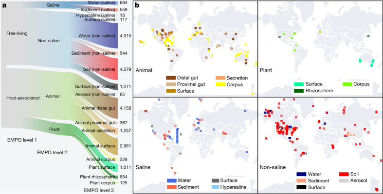
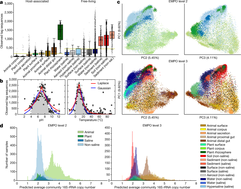
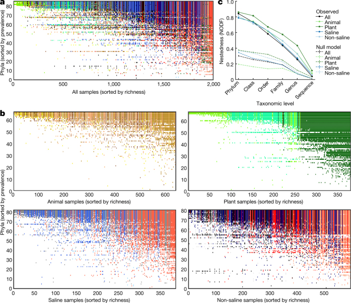
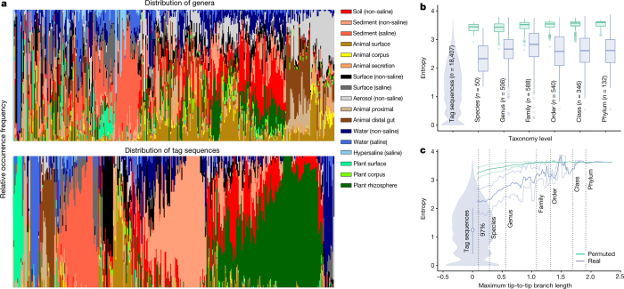
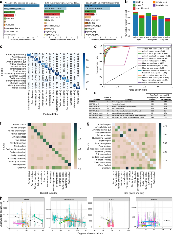
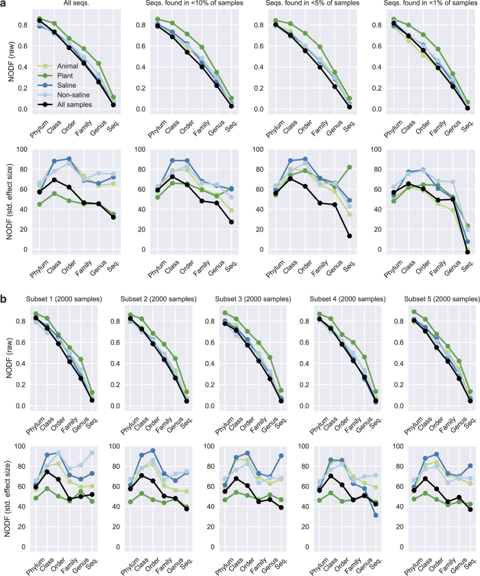
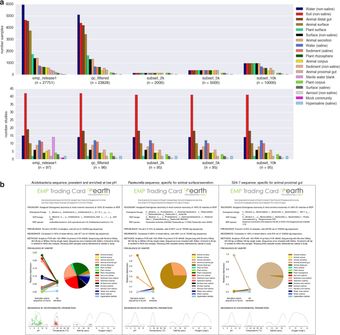
Our growing awareness of the microbial world's importance and diversity contrasts starkly with our limited understanding of its fundamental structure. Despite recent advances in DNA sequencing, a lack of standardized protocols and common analytical frameworks impedes comparisons among studies, hindering the development of global inferences about microbial life on Earth. Here we present a meta-analysis of microbial community samples collected by hundreds of researchers for the Earth Microbiome Project. Coordinated protocols and new analytical methods, particularly the use of exact sequences instead of clustered operational taxonomic units, enable bacterial and archaeal ribosomal RNA gene sequences to be followed across multiple studies and allow us to explore patterns of diversity at an unprecedented scale. The result is both a reference database giving global context to DNA sequence data and a framework for incorporating data from future studies, fostering increasingly complete characterization of Earth's microbial diversity.


Conflict of interest statement

The authors declare no competing financial interests.

Figures

Figure 1
Figure 1. Environment type and provenance of samples.
a, The EMP ontology (EMPO) classifies microbial environments (level 3) as free-living or host-associated (level 1) and saline or non-saline (if free-living) or animal or plant (if host-associated) (level 2). The number out of 23,828 samples in the QC-filtered subset in each environment is provided. EMPO is described with examples at http://www.earthmicrobiome.org/protocols-and-standards/empo. b, Global scope of sample provenance: samples come from 7 continents, 43 countries, 21 biomes (ENVO), 92 environmental features (ENVO), and 17 environments (EMPO). PowerPoint slide Source data
Figure 2
Figure 2. Alpha-diversity, beta-diversity, and predicted average 16S rRNA gene copy number.
a, Within-community (alpha) diversity, measured as number of observed 90-bp tag sequences (richness), in n = 23,828 biologically independent samples as a function of environment (per-environment n shown in Fig. 1a), with boxplots showing median, interquartile range (IQR), and 1.5 × IQR (with outliers). Tag sequence counts were subsampled to 5,000 observations. Yellow line indicates the median number of observed tag sequences for all samples in that set of boxplots. Free-living communities of most types exhibited greater richness than host-associated communities. b, Tag sequence richness (as in a) versus pH and temperature in n = 3,986 (pH) and n = 6,976 (temperature) biologically independent samples. Black points are the 99th percentiles for richness across binned values of pH and temperature. Laplace (two-sided exponential) curves captured apparent upper bounds on microbial richness and their peaked distributions better than Gaussian curves. Greatest maximal richness occurred at values of pH and temperature that corresponded to modes of the Laplace curves. Maximum richness exponentially decreased away from these apparent optima. c, Between-community (beta) diversity among in n = 23,828 biologically independent samples: principal coordinates analysis (PCoA) of unweighted UniFrac distance, PC1 versus PC2 and PC1 versus PC3, coloured by EMPO levels 2 and 3. Clustering of samples could be explained largely by environment. d, 16S rRNA gene average copy number (ACN, abundance-weighted) of EMP communities in n = 23,228 biologically independent samples, coloured by environment. EMPO level 2 (left): animal-associated communities had a higher ACN distribution than plant-associated and free-living (both saline and non-saline) communities. Right: soil communities had the lowest ACN distribution, while animal gut and saliva communities had the highest ACN distribution. PowerPoint slide Source data
Figure 3
Figure 3. Nestedness of community composition.
a, Presence–absence of phyla across samples, with phyla (rows) sorted by prevalence and samples (columns) sorted by richness. Shown is a subset of the EMP consisting of n = 2,000 biologically independent samples with even representation across environments and studies. With increasing sample richness (left to right), phyla tended to be gained but not lost (P < 0.0001 versus null model; NODF (nestedness measure based on overlap and decreasing fills) statistic and 95% confidence interval = 0.841 ± 0.018). b, As in a but separated into non-saline, saline, animal, and plant environments (P < 0.0001, respective NODF = 0.811 ± 0.013, 0.787 ± 0.015, 0.788 ± 0.018 and 0.860 ± 0.021). c, Nestedness as a function of taxonomic level, from phylum to tag sequence, across all samples and within environment types. Also shown are median null model NODF scores (± s.d.). NODF measures the average fraction of taxa from less diverse communities that occur in more diverse communities. All environments at all taxonomic levels were more nested than expected randomly, with nestedness higher at higher taxonomic levels (for example, phyla). PowerPoint slide Source data
Figure 4
Figure 4. Specificity of sequences and higher taxonomic groups for environment.
a, Environment distribution in all genera and 400 randomly chosen tag sequences, drawn from n = 2,000 biologically independent samples with even representation across environments (EMPO level 3) and studies. Each bar depicts the distribution of environments for a taxon (not relative abundance of taxa): bars composed mostly of one colour (environment) are specific for that environment, as seen with tag sequences; bars composed of many colours are more cosmopolitan, as seen with genera. Tag sequences were more specific for environment than were genera and higher taxonomic levels. b, Shannon entropy within each taxonomic group (minimum 20 tag sequences per group) and for the same set of samples with permuted taxonomy labels. Box plots show median, IQR, and 1.5 × IQR (with outliers) for each taxonomic level. A violin plot shows the entropy of tag sequences (minimum 10 samples per tag sequence). Specificity for environment occurred predominantly below the genus level. c, Shannon entropy within phylogenetic subtrees of tag sequences (minimum 20 tips per subtree) defined by maximal tip-to-tip branch length (substitutions per site) and for the same samples with permuted phylogenetic tree tips. Mean and 20th/80th percentile for a sliding window average of branch length is shown. Violin plot for tag sequences as in b. Dotted lines show average tip-to-tip branch length corresponding to 97% sequence identity and taxonomic levels displayed in b. The greatest decrease in entropy was between the lowest branch length subtree tested and tag sequences. PowerPoint slide Source data
Extended Data Figure 1
Extended Data Figure 1. Physicochemical properties of the EMP samples.
Pairwise scatter plots of available physicochemical metadata are shown for temperature, salinity, oxygen, and pH, and for phosphate, nitrate, and ammonium. Histograms for each factor are also shown; the number (n) of samples having data for each factor is provided at the top of each histogram. Samples are coloured by environment, and only QC-filtered samples are included. In sample metadata files, environmental factors are named in our recommended format, with analyte name and units combined in the metadata field name.
Extended Data Figure 2
Extended Data Figure 2. Sequence length, database effects, and beta-diversity patterns.
a, Median sequence length per study after quality trimming. Original EMP studies used 90-bp reads, which were replaced by 100-bp reads for the majority of studies, and have since been replaced by 150–151-bp reads. For most analyses presented in this manuscript, we used the Deblur algorithm and trimmed tag sequences to 90 bp. This allowed inclusion of older studies with shorter read lengths. b, Comparison of Greengenes and SILVA rRNA databases for reference-based OTU picking. Fraction of reads in n = 23,828 biologically independent samples—separated by environment (per-environment n shown in Fig. 1a)—mapping to Greengenes 13.8 and SILVA 123 (97% identity OTUs) with closed-reference OTU picking. Boxplots show median, IQR, and 1.5 × IQR (with outliers). The fraction of reads mapping was similar between Greengenes and SILVA in each environment but slightly higher with SILVA for every environment. c, Alpha-diversity in closed-reference OTUs picked against Greengenes 13.8 and SILVA 123, with sequences rarefied to 100,000, 30,000, 10,000, and 1,000 sequences per sample, displayed as boxplots showing median, IQR, and 1.5 × IQR (with outliers). The sample set for all calculations contained n = 4,667 biologically independent samples having at least 100,000 observations in both Greengenes and SILVA OTU tables. Alpha-diversity metrics were higher with SILVA closed-reference OTU picking than with Greengenes. d, Beta-diversity among all EMP samples using principal coordinates analysis (PCA) of weighted UniFrac distance. Principal coordinates PC1 versus PC2 and PC1 versus PC3 are shown coloured by EMPO levels 2 and 3. As with unweighted UniFrac distance (Fig. 2c), clustering of samples using weighted UniFrac distance could be explained largely by environment.
Extended Data Figure 3
Extended Data Figure 3. Sequence length effects on observed diversity patterns.
The effect of trimming from 150 bp (the approximate starting length of some sequences) to 90 bp (the trimmed length of all sequences in this meta-analysis) was investigated by comparing alpha- and beta-diversity patterns. All samples, at each sequence length, were rarefied to 5,000 sequences per sample. a, Alpha-diversity distributions of n = 12,538 biologically independent samples displayed as histograms of observed tag sequences coloured by environment (EMPO level 3). Among these samples with sequence length ≥ 150 bp, the distributions are largely preserved when trimming from 150 to 100 to 90 bp. b, Procrustes goodness-of-fit between the 90-bp (grey lines) and 150-bp (black lines) Deblur principal coordinates (unweighted UniFrac distance) for n = 200 randomly chosen samples coloured by environment (EMPO level 2). Beta-diversity patterns between the two sequence lengths are similar.
Extended Data Figure 4
Extended Data Figure 4. Tag sequence prevalence patterns.
Note that for this meta-analysis, the input observation table was filtered to keep only tag sequences with at least 25 observations total over all samples and then rarefied to 5,000 observations per sample. a, Per-study endemism visualized as a histogram of tag sequences binned by the number of studies in which they are observed (right: linear scale; left: log scale). b, Per-sample endemism visualized as a histogram of tag sequences binned by the number of samples in which they are observed (right: sample counts up to 92 samples and the number of tag sequences in linear scale; left: all tag sequences with bin widths of 100 samples and number of tag sequences in log scale). c, Abundance (total observations in rarefied table) versus prevalence (number of samples observed in) of n = 307,572 tag sequences. Both axes are log scale. The most prevalent tag sequences were also the most abundant. d, Prevalence as a function of sequencing depth in n = 2,279 soil, n = 478 saltwater, n = 1,508 freshwater, and n = 695 animal distal gut samples having at least 50,000 sequences per sample. Shown are the average and s.d. of mean prevalence across triplicate rarefied subsamples of 50, 100, 500, 1,000, 5,000, 10,000, and 50,000 sequences per sample. Average prevalence increases with sequencing depth, and the straight-line relationship on the log–log axis is suggestive of a power law. e, Histograms of tag sequence prevalences at each sampling depth. The histograms show the distribution moving towards higher prevalences with increasing sequencing depth. Gut data lacked tag sequence prevalences > 0.7 owing to the inclusion of very different host species; see f. f, Histograms as in e but on a subset of the observation tables where 30 samples were randomly sampled from each study. Restricting to human gut samples only, the full range of prevalences found in the other environments is observed.
Extended Data Figure 5
Extended Data Figure 5. Environmental effect sizes, sample classification, and correlation patterns.
a, Effect sizes of predictors on alpha- and beta-diversity. Maximum pairwise effect size (difference between means divided by standard deviation) between categories of each predictor plotted for observed tag sequences (alpha-diversity) and unweighted and weighted UniFrac distance (beta-diversity). Response variables (alpha- and beta-diversity) were derived from the QC-filtered subset of the 90-bp Deblur table containing n = 23,828 biologically independent samples. Numeric predictor variables were converted to quartiles (categorical predictors). Categories within each predictor had a minimum of 75 samples per category. b, Cumulative variation explained by the optimal model of stepwise redundancy analysis (RDA) of predictors: study ID, EMPO level 3, ENVO biome level 3, latitude, and longitude (predictors with values for less than half of samples, including host scientific name, were excluded). Environment (EMPO level 3) and biome (ENVO biome level 3) explained as much variation as study ID when study ID was excluded from the RDA. c, Confusion matrix for random forest classifier of samples to environment (EMPO level 3). The classifier was trained on the 2,000-sample subset, which was then tested on the remaining samples (QC-filtered samples minus 2,000-sample subset). Squares are coloured relative to 100 classification attempts for each true label. Overall success rate was 84%, with the most commonly misclassified sample environments being Surface (non-saline), Animal secretion, Soil (non-saline), and Aerosol (non-saline). d, Receiver operating characteristic (ROC) curve for classification of samples to environment (EMPO level 3). The AUC (area under curve) indicates the probability that the classifier will rank a randomly chosen sample of the given class higher than a randomly chosen sample of other classes. e, Classification success, using a random forest classifier, to EMPO levels 1–3, ENVO material, ENVO feature, and ENVO biome levels 1–3. f, Microbial source tracking: mean predicted proportion of tag sequences from each source environment (EMPO level 3) that occurs in each sink environment. The model was trained on a subset of samples (~20% of each environment), and tested to predict tag sequence source composition in all remaining samples. Aerosol (non-saline), Surface (saline), and Hypersaline samples were not included in this analysis because there were insufficient sample numbers. g, Microbial source tracking: which other environments a sample type most resembles. The model was trained on all source environments except one using a leave-one-out cross-validated model, and then used to classify each sample included in that group. Hence, the predicted classification proportion of environment X to environment X is zero. h, Correlation of microbial richness with latitude. Richness of 16S rRNA tag sequences per sample across EMPO level 2 environmental categories as a function of absolute latitude. Samples from studies that span at least 10° latitude are highlighted in colour, with linear fits displayed per-study as matching coloured lines. Samples from studies with narrower latitudinal origins are shown in grey. The global fit for all samples per category is indicated by a dashed black line.
Extended Data Figure 6
Extended Data Figure 6. NODF scores of nestedness across samples by taxonomic level.
The NODF statistic represents the mean, across pairs of samples, of the fraction of taxa occurring in less diverse samples that also occur in more diverse samples. A raw NODF of 0.5 would mean that for any pair of samples, on average 50% of the taxa in the less diverse sample would occur in the more diverse sample. a, NODF (raw) and NODF standardized effect size in the 2,000-sample subset by taxonomic level. Results are shown first for all tag sequences and then for tag sequences found in <10%, < 5%, and <1% of samples. By removing the most prevalent tag sequences before analysis (and rarefying only after this step), it was possible to rule out artefacts associated with potential contamination. NODF (raw) is highest at the phylum level and decreases at finer taxonomic levels, and this trend is observed even when the most prevalent tag sequences are removed (removing those occurring in ≥ 10%, ≥ 5%, or ≥ 1% of samples). The decreasing trend is likely to be partially due to finer taxonomic groups having lower prevalence (and lower matrix fill, among other factors) than coarser taxonomic groups, as standardized effect sizes of the NODF statistic are essentially constant across taxonomic levels. b, When five alternate 2,000-sample subsets are randomly drawn (with replacement) from the full (QC-filtered) EMP dataset, the trends in NODF (raw) and NODF standardized effect size remain largely unchanged.
Extended Data Figure 7
Extended Data Figure 7. Subsets and EMP trading cards.
a, Subsets of the EMP dataset with even distribution across samples and studies. Shown are all EMP samples included in this manuscript (release 1), the QC-filtered subset, and subsets of 10,000, 5,000, and 2,000 samples. The latter three contain progressively more even representation across environments and studies, providing a more representative view of the Earth microbiome and a more lightweight dataset. Top, histograms of samples per environment (EMPO level 3) for each subset. Bottom, histograms of studies per environment (EMPO level 3) for each subset. b, EMP trading cards: distribution of 16S rRNA tag sequences across the EMP. Trading cards highlight the power of the EMP dataset to help define niche ranges of individual microbial sequence types across the planet’s microbial communities. Cards show distribution of 16S rRNA tag sequences in a 2,000-sample subset of the EMP (rarefied to 5,000 observations per sample) having even distribution by environment (EMPO level 3) and study. Taxonomy is from Greengenes 13.8 and Ribosomal Database Project (RDP), with the fraction of exact RDP matches by lineage and species name shown in parentheses. The pie chart and point plot show the relative distribution of environments in which the tag sequence is found (left points) versus the environment distribution of all 2,000 samples (right points). The coloured scatter plots indicate tag sequence relative abundance (normalized to the shared y axis) as a function of metadata values (no points shown indicates that metadata were not provided for that category). For comparison, grey curves with rug plots indicate kernel density estimates of metadata values across all samples in the set of 2,000 (not just samples where the tag sequence was found). Three examples are shown. Left, a prevalent sequence enriched in soil and plant rhizosphere is from the class Acidobacteria, aptly named as this sequence is found at highest relative abundance in low-pH samples. Middle, the sequence most specific for animal surface (also enriched in animal secretion) is annotated as Pasteurella multocida, a common cause of zoonotic infections following bites or scratches by domestic animals, such as cats and dogs. Right, the sequence most specific for animal proximal gut belongs to S24-7, a family highly localized to the gastrointestinal tracts of homeothermic animals and predominantly found in herbivores and omnivores, but not in carnivores.

References

    1. Lozupone CA, Knight R. Global patterns in bacterial diversity. Proc. Natl Acad. Sci. USA. 2007;104:11436–11440. - PMC - PubMed
    1. Ley RE, Lozupone CA, Hamady M, Knight R, Gordon JI. Worlds within worlds: evolution of the vertebrate gut microbiota. Nat. Rev. Microbiol. 2008;6:776–788. - PMC - PubMed
    1. Fierer N, Jackson RB. The diversity and biogeography of soil bacterial communities. Proc. Natl Acad. Sci. USA. 2006;103:626–631. - PMC - PubMed
    1. Steele JA, et al. Marine bacterial, archaeal and protistan association networks reveal ecological linkages. ISME J. 2011;5:1414–1425. - PMC - PubMed
    1. Philippot L, Raaijmakers JM, Lemanceau P, van der Putten WH. Going back to the roots: the microbial ecology of the rhizosphere. Nat. Rev. Microbiol. 2013;11:789–799. - PubMed

Publication types

Substances