Highly scalable multichannel mesh electronics for stable chronic brain electrophysiology

Abstract

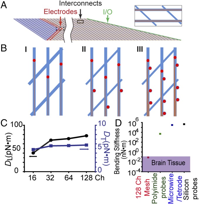
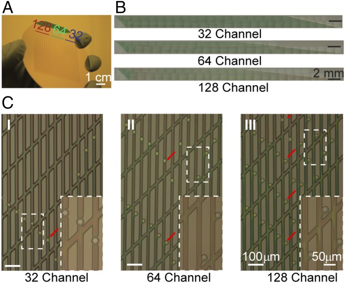
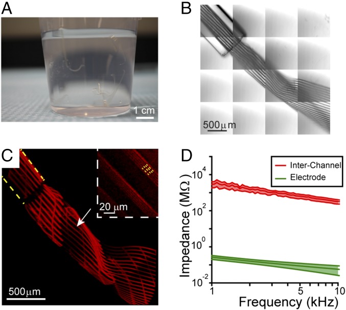
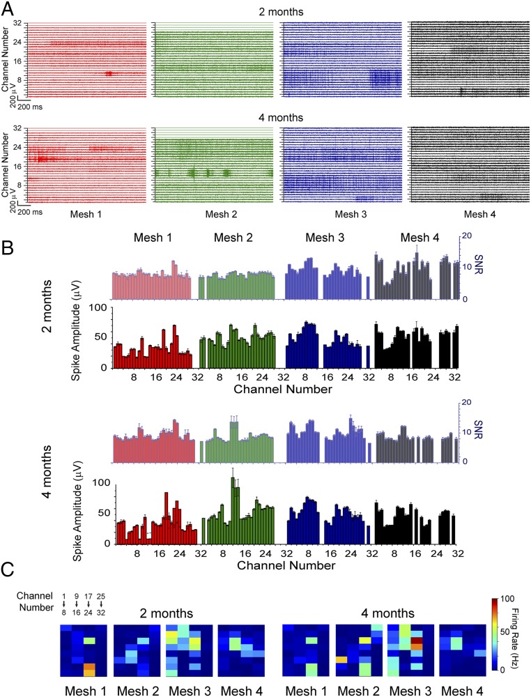
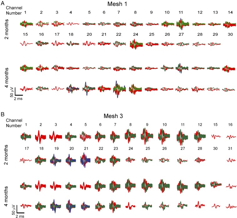
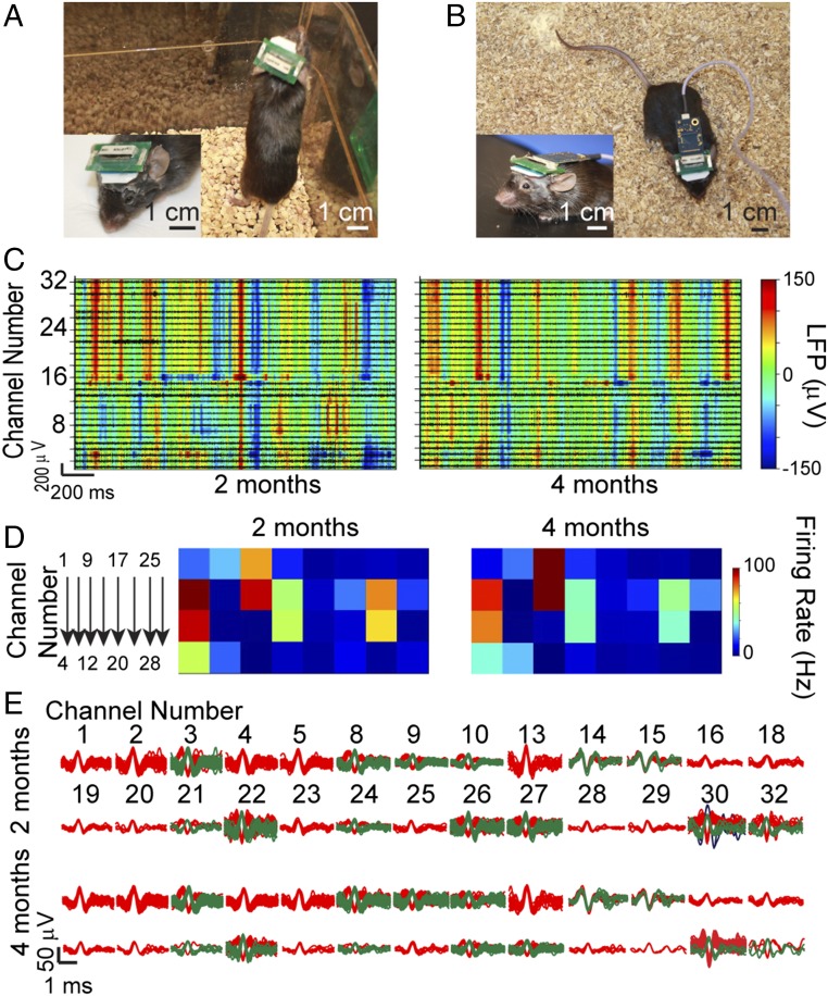
Implantable electrical probes have led to advances in neuroscience, brain-machine interfaces, and treatment of neurological diseases, yet they remain limited in several key aspects. Ideally, an electrical probe should be capable of recording from large numbers of neurons across multiple local circuits and, importantly, allow stable tracking of the evolution of these neurons over the entire course of study. Silicon probes based on microfabrication can yield large-scale, high-density recording but face challenges of chronic gliosis and instability due to mechanical and structural mismatch with the brain. Ultraflexible mesh electronics, on the other hand, have demonstrated negligible chronic immune response and stable long-term brain monitoring at single-neuron level, although, to date, it has been limited to 16 channels. Here, we present a scalable scheme for highly multiplexed mesh electronics probes to bridge the gap between scalability and flexibility, where 32 to 128 channels per probe were implemented while the crucial brain-like structure and mechanics were maintained. Combining this mesh design with multisite injection, we demonstrate stable 128-channel local field potential and single-unit recordings from multiple brain regions in awake restrained mice over 4 mo. In addition, the newly integrated mesh is used to validate stable chronic recordings in freely behaving mice. This scalable scheme for mesh electronics together with demonstrated long-term stability represent important progress toward the realization of ideal implantable electrical probes allowing for mapping and tracking single-neuron level circuit changes associated with learning, aging, and neurodegenerative diseases.

Keywords: large-scale neural recording; nano−bio interface; neural probe; tissue-like; ultraflexible.

Fig. 1.

Scalable scheme for high-density multiplexed mesh electronics. (A) Scheme showing a 64-channel scalable highly multiplexed mesh electronics probe with 32 longitudinal elements. Two individually addressable metal interconnects (orange lines) are incorporated in each longitudinal element (Inset) connecting recording electrodes (red circles) at one end and I/O pads (green circles) at the other end. The dashed and solid black boxes highlight the electrodes and interconnects region shown in B, II (rotated 90°) and Inset, respectively. (B) Schematics showing scaling of channel number and recording site density via incorporation of multiple channels in a single longitudinal element. Red circles, orange lines, and blue mesh structures represent the Pt microelectrodes, Au interconnects, and SU-8 mesh ribbons, respectively. (C) Simulated longitudinal (black, left y axis) and transverse (blue, right y axis) bending stiffness values for the 16-, 32-, 64-, and 128-channel mesh designs. The 16-channel mesh has the same structure as reported previously (33) (see Materials and Methods and SI Text for simulation details). (D) Comparison of the bending stiffness of 128-channel mesh electronics (red square) with that of brain tissue (purple rectangle) and those of conventional implantable electrical probes: planar polyimide probes (39) (green square), microwire or tetrode (18) (blue square), and silicon probes (black square) (40).

Fig. 2.

High-density multiplexed mesh electronics via standard PL. (A) Photograph showing fabricated 32-, 64-, and 128-channel mesh designs on a 3-inch (76.2 mm) diameter silicon wafer before dissolution of the Ni sacrificial layer. A total of 21 mesh electronics probes with 7 of each channel design were fabricated on the wafer. (Scale bar: 1 cm.) (B) Stitched bright field microscope images showing fabricated 32- (Upper), 64- (Middle), and 128-channel (Lower) mesh electronics probes on a silicon wafer. Recording electrodes and I/O pads are located at the left and right, respectively, of the images. Each stitched image comprises ca. 50 wide-field microscope images (1.35 mm × 1.70 mm for each image) taken under 5× magnification. (Scale bars: 2 mm.) (C) Bright-field microscope images showing scaling up of channel number and recording site density via fabricating multiple (1, 2, and 4 in I, II, and III, respectively) channels in a single longitudinal element. The red arrows highlight the number of recording sites (Pt microelectrodes) on a single longitudinal element. Insets present zoom-in views of the white dashed boxes. [Scale bars: 100 μm and 50 μm (for Inset).]

Fig. 3.

Imaging and electrical characterization of highly multiplexed mesh electronics. (A) Photograph of seven free-standing 128-channel mesh electronics with the design shown in Fig. 2C, III suspended in water. The mesh electronics were transferred by glass needles after being released from the silicon wafer. (Scale bar: 1 cm.) (B) DIC image of a 128-channel mesh electronics injected through a 400-μm ID glass needle into water. The image was acquired in 4 × 4 Tile Scan mode with each of the tiles having a field of view of 850 μm × 850 μm, and the total image is 3,400 μm × 3,400 μm. (Scale bar: 500 μm.) (C) A 3D reconstructed confocal image of a rhodamine-6G labeled 128-channel mesh electronics injected into water via a 400-μm ID needle (yellow dashed line). The image was acquired in 4 × 4 Tile Scan with each of the tile components having a field of view of 850 μm × 850 μm, and the total image size is 3,400 μm × 3,400 μm. The white arrow highlights the region of the mesh that is zoomed in and shown in Inset from a different viewing angle. (Scale bar: 500 μm.) (Inset) A magnified image of a single plane confocal image (3 μm focal depth) showing the four Au interconnect lines, which appear as dark lines, in each longitudinal mesh element (running upper left to lower right); in the upper right longitudinal element, yellow dashed lines highlight the positions of four Au interconnect lines. (Scale bar: 20 μm.) (D) Average impedance values between adjacent Au interconnects (2 μm edge-to-edge distance) on the same longitudinal elements of the 128-channel mesh design (red) and those of the Pt microelectrodes (20-μm diameter) of the same mesh probe measured in the frequency range of 1 kHz to 10 kHz. The averages were obtained over 10 pairs of adjacent Au interconnects and 10 Pt microelectrodes (SI Text). The shaded areas indicate ±1 SD with a sample size N = 10.

Fig. 4.

Multisite injections of mesh electronics. (A) Schematic, (B) photo, and (C) micro-CT image showing four mesh electronics (yellow arrows) injected into the same mouse. Four FFCs were stacked both vertically and horizontally for I/O connections during surgery. A, P, D, and V in C correspond to the anterior, posterior, dorsal, and ventral directions, respectively. (D) Photo of a freely behaving mouse with four meshes injected. (Scale bars: 1 cm in B and D; 2 mm in C.)

Fig. 5.

Simultaneous 128-channel chronic recordings. (A) Band-pass (250 Hz to 6,000 Hz) filtered extracellular spike recordings from four 32-channel meshes injected into the same mouse at 2 (Upper) and 4 (Lower) mo postinjection. Meshes 1 (red) and 2 (green) were injected into the motor CTX, and meshes 3 (blue) and 4 (black) were injected into the HIP. (B) Bar charts showing average SNR (lighter colors, right y axis) and spike amplitude (darker colors, left y axis) from all channels at 2 (first and second rows) and 4 (third and fourth rows) mo postinjection. The color codes of different meshes are consistent with those in A. The error bars indicate the SEM, with sample size N equal to the total number of sorted spikes of the corresponding channel. See SI Text for details of SNR estimation. (C) Average firing rate maps of all channels at 2 (Left) and 4 (Right) mo postinjection. Colors indicate firing rate based on the color bar on the right.

Fig. 6.

Spike sorting analyses of chronic recordings. Overlay of sorted and clustered spikes from all channels with identifiable spikes for (A) mesh 1 and (B) mesh 3 in Fig. 5 at 2 mo (Upper) and 4 mo (Lower) postinjection. The channel numbers are specified above the corresponding sorted spikes for 2 mo and remain the same for 4 mo.

Fig. 7.

Chronic recordings from freely behaving mouse. (A) Photograph of a typical freely behaving mouse with low-profile FFC and PCB when housed in animal facility. (B) Photograph of typical freely behaving mouse during recording. Voltage amplifier was directly positioned near the mouse head to minimize mechanical noise coupling. A flexible serial peripheral interface cable (light purple) was used to transmit amplified signals to the data acquisition systems. (Insets) Zoom-in views of the electrical connections on mouse head. (Scale bars: 1 cm.) (C) Representative 32-channel LFP (heat maps) with amplitudes color-coded according to the color bar on the far right and extracellular spikes (traces) mapping from the same mouse at 2 (Left) and 4 (Right) mo postinjection. The x axes show the recording time, and the y axes represent the channel number of each recording electrode. (D) Average spike firing rate maps of all channels at 2 (Left) and 4 (Right) mo postinjection. The channel numbers are specified on the left. Colors indicate firing rate based on the color bar on the right. (E) Sorted spikes from all 26 channels with identifiable spikes at 2 (first and second rows) or 4 (third and fourth rows) mo postinjection for recordings in C. The channel numbers are specified above the corresponding sorted spikes for 2 mo and remain the same for spikes recorded at 4 mo.

References

1. Buzsáki G. Large-scale recording of neuronal ensembles. Nat Neurosci. 2004;7:446–451. - PubMed
1. Stanley GB. Reading and writing the neural code. Nat Neurosci. 2013;16:259–263. - PubMed
1. Bargmann CI, Newsome WT. The Brain Research through Advancing Innovative Neurotechnologies (BRAIN) initiative and neurology. JAMA Neurol. 2014;71:675–676. - PubMed
1. Harris KD, Quiroga RQ, Freeman J, Smith SL. Improving data quality in neuronal population recordings. Nat Neurosci. 2016;19:1165–1174. - PMC - PubMed
1. Borchers S, Himmelbach M, Logothetis N, Karnath HO. Direct electrical stimulation of human cortex—The gold standard for mapping brain functions? Nat Rev Neurosci. 2011;13:63–70. - PubMed
Publication types