Fully integrated silicon probes for high-density recording of neural activity

Abstract

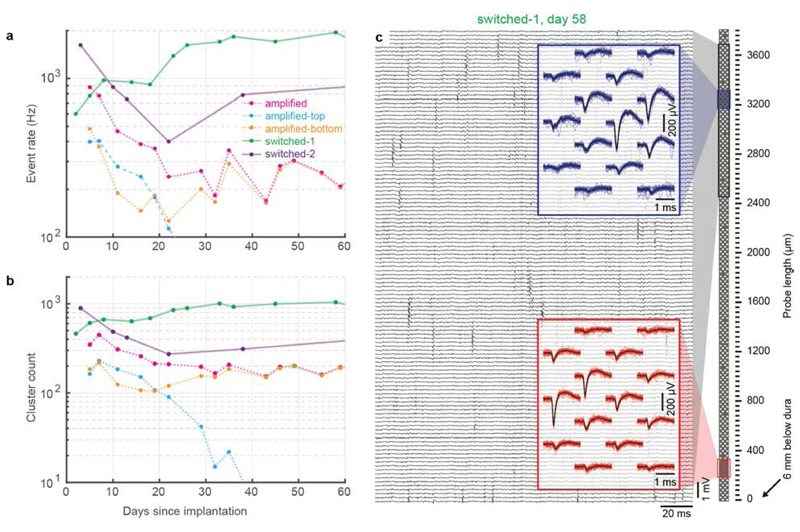
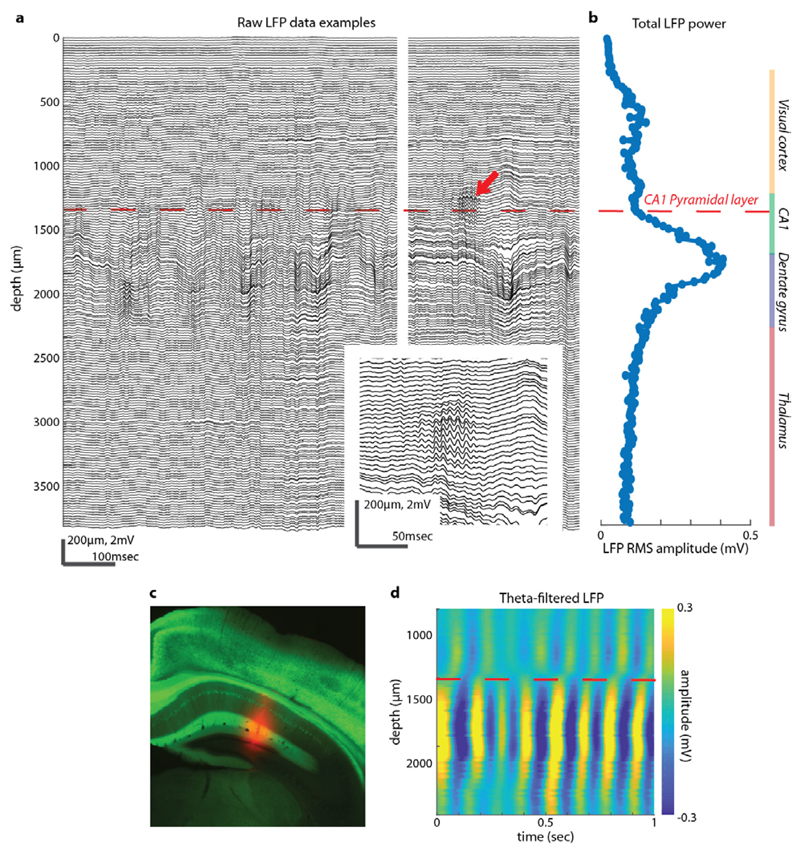
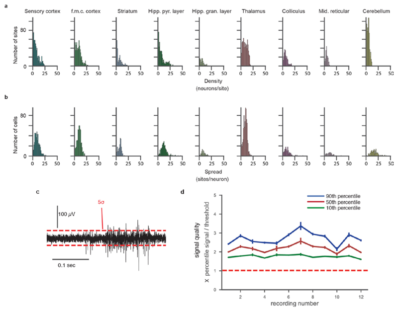
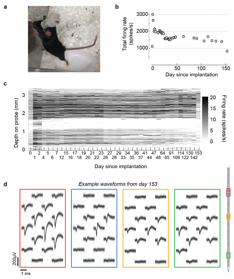
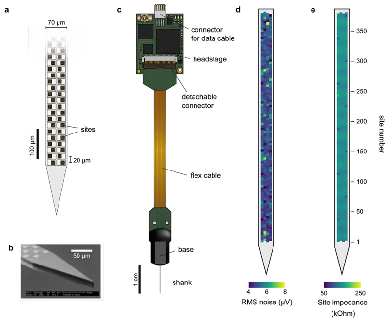
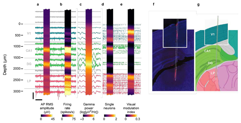
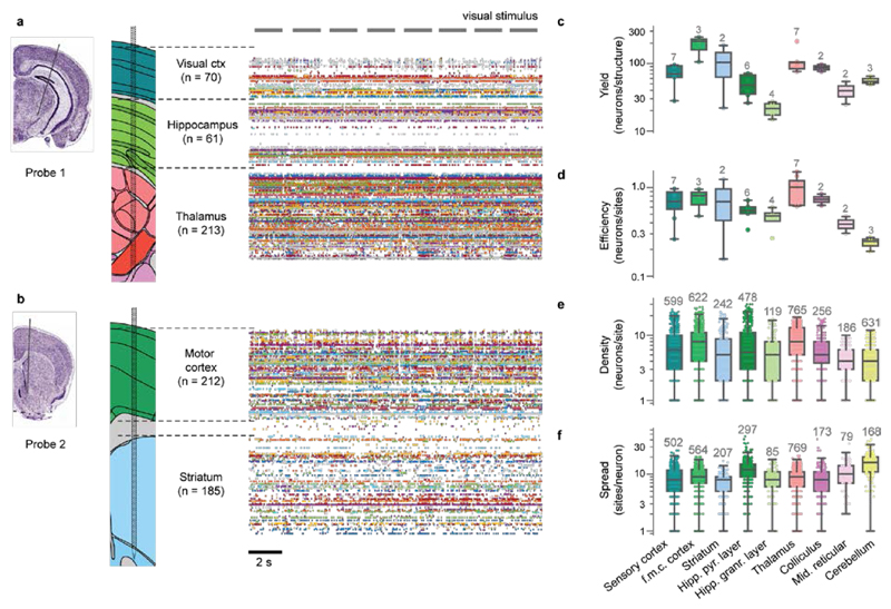
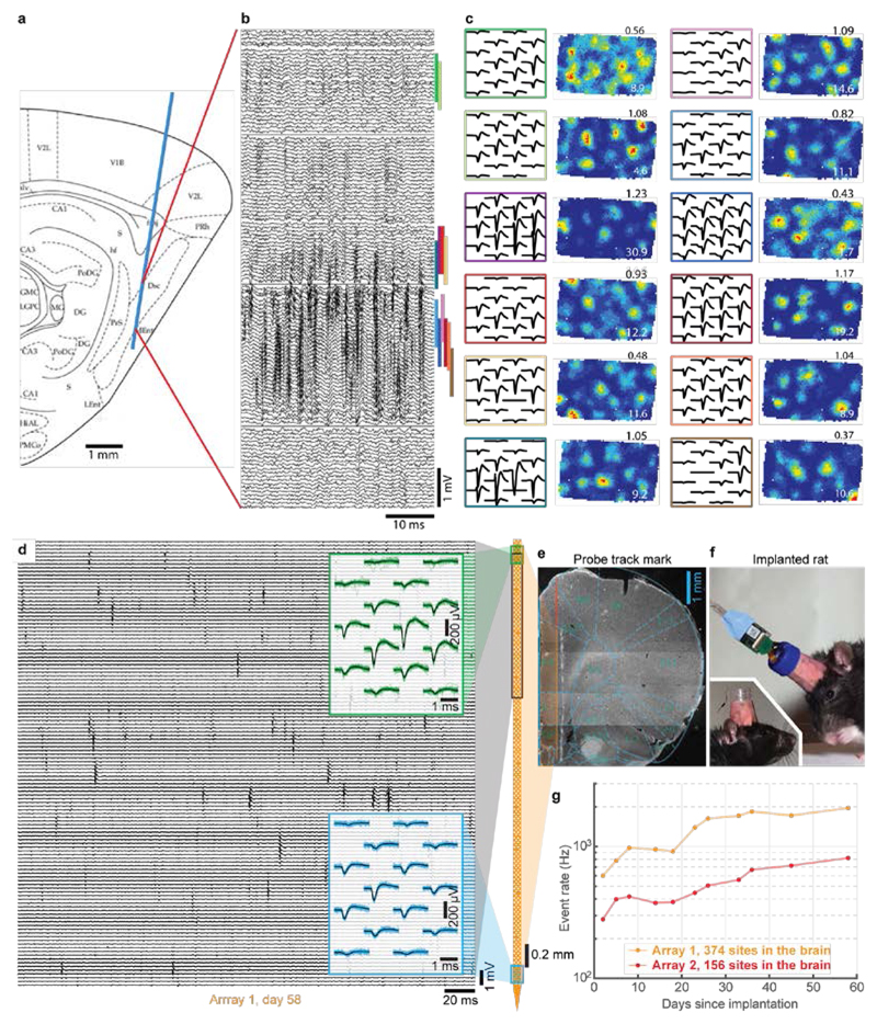
Sensory, motor and cognitive operations involve the coordinated action of large neuronal populations across multiple brain regions in both superficial and deep structures. Existing extracellular probes record neural activity with excellent spatial and temporal (sub-millisecond) resolution, but from only a few dozen neurons per shank. Optical Ca²⁺ imaging offers more coverage but lacks the temporal resolution needed to distinguish individual spikes reliably and does not measure local field potentials. Until now, no technology compatible with use in unrestrained animals has combined high spatiotemporal resolution with large volume coverage. Here we design, fabricate and test a new silicon probe known as Neuropixels to meet this need. Each probe has 384 recording channels that can programmably address 960 complementary metal-oxide-semiconductor (CMOS) processing-compatible low-impedance TiN sites that tile a single 10-mm long, 70 × 20-μm cross-section shank. The 6 × 9-mm probe base is fabricated with the shank on a single chip. Voltage signals are filtered, amplified, multiplexed and digitized on the base, allowing the direct transmission of noise-free digital data from the probe. The combination of dense recording sites and high channel count yielded well-isolated spiking activity from hundreds of neurons per probe implanted in mice and rats. Using two probes, more than 700 well-isolated single neurons were recorded simultaneously from five brain structures in an awake mouse. The fully integrated functionality and small size of Neuropixels probes allowed large populations of neurons from several brain structures to be recorded in freely moving animals. This combination of high-performance electrode technology and scalable chip fabrication methods opens a path towards recording of brain-wide neural activity during behaviour.

Extended Data Figure 1. Comparison of switchable and active probe options.

a, Cumulative distribution of the single unit peak amplitude from recordings using non-switchable (option 1, blue, n=5 recordings) or switchable (option 3, green, n=5 recordings) probes. Each distribution shows an individual recording session; sessions were spike sorted, and the mean waveform on every channel for each unit was computed. The largest absolute peak in the mean waveform on any channel was taken as the amplitude. b, Distribution of mean firing rate across the recording sessions for each sorted unit from non-switchable (blue, n = 119 cells) and switchable (green, n = 294 cells) probes; all recordings with each variant are combined. Switches did not have an appreciable effect on the amplitude or firing rate of recorded units. c, Artifacts in awake head-fixed locomoting mice are similar across passive and active probe options and can be removed by common (median) average referencing. Filtered traces (bandpass 300 to 3000 Hz) of 4 channels sampled at different depths (gray) and corrected common average referenced (CAR) traces (red). The CAR corrected traces are obtained by subtracting from each trace the median across all 120 channels (bottom). Figure panel depicts representative examples of artifacts found on both probe options. d, Extracellular spike waveform amplitude (signal), noise amplitude, and spike signal-to-noise ratio measured in cortex in vivo using passive (black) or actively amplified (red) recording sites. Voltage amplitudes are sampled from 250,000 spikes across the entire probe for each experiment (4 experiments with passive (SNR=8.78 ± 0.52, 95% confidence interval) and 4 with active (SNR=8.95 ± 0.54) recording sites). Signal-to-noise (right) distributions are similar - wilcoxon rank-sum; p-value 0.78, two-sided. e,f, Signal-to-noise ratio computed using 200,000 spikes during locomotion (red) or stationary (black) epochs. Recordings with passive sites (3 recordings) are depicted in e and recordings with active sites (4 recordings) in f. SNR distributions are similar during stationary and locomotion epochs with both probe options. Overall, the performance of probes with on-site buffer amplification is similar to that of probes with passive sites and offers no clear advantage in vivo.

Extended Data Figure 2. Impact and chewing transient rejection.

Reduction of interfering transients with common average reference (CAR) post-processing in software. Recordings using external reference on one animal, 6 or 12 trials for each technology option. a, Example signal traces for a phase 3 unbuffered, switched probe in a chronically implanted rat tapped with a cable tie. Shown is the median across all 374 recording sites (red), the raw traces (gray, from 4 adjacent sites), and traces corrected with local CAR (blue; see Methods). b, Impact transient magnitudes for all 4 probe options chronically implanted with external referencing, and corrected with global or local CAR (n=6 trials, one animal, median±interquartile range). Probes with unity gain buffer amplifiers at the sites (Opt. 2 & 4) offer no significant advantage for CAR-processed data over probes without buffers (Opt. 1 & 3). c, Transients as in a, induced by chewing food, and d, comparison of all 4 options as in b. Same trial counts, one animal. Again, there was no significant advantage to buffer amplifiers after CAR correction (two-sample t-test, P=0.1266, α=0.05, one-tailed). The median and interquartile ranges are computed from 12 chewing events measured at 270 sites (Opt. 4) or 374 sites (Opts. 1, 2, & 3). n in b and d represents the number of independent samples (number of sites x number of trials). See Methods for details.

Extended Data Figure 3. Light sensitivity tests.

a,b, A comparison of the light sensitivity of active and passive Neuropixels probes, along with “conventional” Si probes. a, Plot of transient amplitude vs. illumination power density for a 5 ms directly-applied 473nm light pulse. Active sites, especially unswitched were most sensitive. Switched and unswitched passive probes were much less sensitive. In each measurement a 5 ms light pulse was applied singly or in a pulse train at 20 Hz for 1 sec. b, Example response to illumination with a 5 ms pulse at the indicated power density. In all cases, probes were illuminated with light from a 100 μm core multimode fiber with the probe immersed in 1X phosphate buffered saline. Below intensities of 10-20 mW/mm² directly onto the probe, there is no impact on spike detection (see Extended Data Figure 8) or LFP phase or magnitude determination for passive switched Neuropixels probes. Experiments in a,b were performed once for each probe type. c-e, Neuropixels recording sites were immersed in saline and directly illuminated with blue (465 nm) LED light from a 200 micron diameter, 0.66 NA fiber optic cable. Light was delivered with 6 different pulse shapes (ramp, raised cosine, square 1 ms, 10 ms, 100 ms, and 1 s) at 3 peak power levels. c, Light power measured with an amplified photodetector for all 18 pulse types. d,e, Artifacts on a representative channel for low (cyan traces), middle (magenta traces), and high (yellow traces) light levels. For reference, the input range of the LFP band (gain of 250x) is overlaid across the LFP plots.

Extended Data Figure 4. Long-term stability studies: Effects of shank width, TiN sites, and active and switched sites.

a-d, To compare the chronic performance of 50 μm wide and 70 μm wide shanks as well as TiN and PEDOT-coated gold sites, 4-shank probes with 2 shanks of each width were fabricated. One version had PEDOT-coated gold sites and a second had TiN sites. These were tested in separate animals. a, A diagram of the probe geometry for both probes, two of 4 shanks, a photograph of the distal end of a TiN site shank, and an electron microscopy image of one TiN site. The site is 12×12 μm. These probes were chronically implanted in rat medial prefrontal cortex (mPFC) and recorded in unrestrained animals, without advancing the electrodes, in multiple sessions over a period of 6-8 weeks (further implantation, recording, and analysis details are described in the Methods). b, The event rate vs implant age for one of two rats with TiN probes in mPFC. We define an event as time-coincident spikes recorded on a contiguous group of sites for which the maximum amplitude on any site in the group exceeds the threshold. c, The event rate vs implant age for four rats with one probe each in mPFC: two animals with TiN site probes, two animals with Gold:PEDOT site probes. Differences in behavioral state likely contribute to the variability in event rate. d, The event SNR, defined in the Methods. The stability of this signal quality metric suggests that the drop in event rate for PEDOT-1 was due to biological factors unrelated to probe site integrity. e-g, Probes (Phase 2) of all four shank designs, passive, active, passive switched, and active switched were implanted chronically in rat mPFC. Recordings were made at least once per week. Data analysis, implant method, and recording procedures are described in detail in the supplementary text. There is no apparent downward trend in neural activity by either metric (e,f), thus all four shank technologies can achieve exceptional chronic stability. g, mPFC recording, 200 ms of activity traces and examples of waveforms from two sorted units. Insets: Dark lines show average waveform overlaid with 30 randomly selected single event waveforms of a neuron located at the top (green) and bottom (red) of the most distal group of 128 sites.

Extended Data Figure 5. Stability of chronically implanted Phase 3 active and switched probe technologies in rats.

a,b, Phase 3 fully integrated probes: two of four designs were implanted in mPFC of rats as for Phase 2 (Extended Data Figure 4). One probe with amplified sites and two switchable, un-amplified probes (the preferred technology) were implanted. Amplified, switchable probes were implanted but were damaged electronically before adequate recording data could be accumulated. There was no indication of activity loss over the 8 weeks of recording (linear regression t-test, one-tailed, P>0.1) except for the top half of one probe (blue). This good performance was expected based on Phase 2 results, but the active and active switched probes are 70 μm wide in Phase 3 compared to 50 μm wide for Phase 2. See supplementary text for details of data analysis, implant method, and recording procedures. We define an event as time-coincident spikes recorded on a contiguous group of sites for which the maximum amplitude on any site in the group exceeds the threshold. Across a population of 14 probes chronically implanted in rat mPFC (Phases 2 and 3), we did not observe degradation of spiking activity over 8 weeks (linear regression t-test, single-tailed, P>0.1, n=30 sessions). The sole exception to this observation is shown in a and b above (blue). In this case, the upper half of the distal most 3.8 mm array lost nearly all activity over the first 30 days while the lower ~1.9 mm remained stable for the duration of the 8 weeks monitored. A few probe implants became detached from the skull after many months (3 of 16 implants, 223-482 days) or surgery wound irritation required the subject animal to be euthanized (but always after >20 weeks). c, mPFC recording, 200 ms of activity traces and examples of waveforms from two sorted units. Insets: Dark lines show average waveform overlaid with 30 randomly selected single event waveforms of a neuron located at the top (blue) and bottom (red) of the distal most group of 384 sites.

Extended Data Figure 6. Further examples of LFP data quality.

a, Two example periods of LFP data, over the entire depth of the probe. The data were filtered with a third-order Butterworth low-pass filter with 300 Hz cutoff frequency, but otherwise unprocessed. Only one channel from each depth along the probe is shown, so the total number of plotted traces is 192 rather than 384. Left example shows an epoch without ripples, and right example shows an epoch with a ripple (indicated by red arrow). The ripple is expanded in the inset. b, Quantification of LFP signal amplitude (root mean square) across depth. At right, the anatomical locations of the sections of the probe are depicted, which were determined from histology, part of which is shown in panel c, along with functional markers such as spike rates and amplitudes. c, Histological section depicting the location of the probe (stained with DiI) as it passed through hippocampus. d, Theta-filtered LFP. The same data from panel a (left) were filtered with a third-order bandpass Butterworth filter between 4 and 10 Hz, and are here depicted as a colormap to emphasize the phase inversion at the CA1 pyramidal layer (indicated by red dashed line).

Extended Data Figure 7. Spike band signal quality across brain areas and multiple acute recordings.

a, For each channel in each brain area, the number of neurons with a mean waveform >20µV was counted (‘density’). b, For each neuron recorded in each brain area, the number of channels on which that neuron produces a mean waveform >20 µV (‘spread’) was counted.In a separate set of experiments, the same probe was used for a series of 12 acute in vivo recordings in 10 animals across 4 months. c, The signal quality of each recording was computed by measuring the amplitude of detected spikes relative to the detection threshold within a 30 second selection of the recording. The detection threshold used was always 5 times the standard deviation (σ) of the mean signal. d, The mean (+/- SEM, n=200) ratio of the 90th percentile (blue), 50th percentile (red) and 10th percentile (green) to the 5σ detection threshold across all channels with an event, for each recording.

Extended Data Figure 8. Recording during optogenetic stimulation of excitatory and inhibitory cell populations.

a,b, A Neuropixels probe was inserted into primary visual cortex of a Rorb-Cre;Ai32 mouse expressing ChR2 in Rorb-positive cells, which are primarily excitatory neurons of layer 4. Stimulation was carried out with a 465 nm LED coupled to a 200 micron, 0.66 NA fiber optic cable placed on the surface of the cortex approximately 1 mm from the recording site. Each trial (N = 20) consisted of a raised cosine light pulse 1 s in duration, with a peak intensity of 300 mW/mm². a, Average multiunit firing rate across 250 channels, aligned to the start of the optogenetic stimulus. Location of the brain surface is marked with a white line. b, Average LFP band response to the optogenetic stimulus for 125 channels along the left edge of the probe (a subset of the sites in panel a). c,d, A Neuropixels probe was inserted into primary visual cortex of a PV-Cre;Ai32 mouse expressing ChR2 in PV-positive cells, which are primarily fast-spiking inhibitory neurons. Stimulation was carried out with a 470 nm laser focused to a ~150 µm diameter spot on the surface of the cortex at the recording site. Each trial (N = 15) consisted of a 500 ms, 40 Hz raised cosine light pulse, with a peak intensity of 25 mW/mm². c, Average multiunit firing rate (regular-spiking waveforms only) across 150 channels, aligned to the start of the optogenetic stimulus. Location of the brain surface is marked with a white line. d, Average LFP band response to the optogenetic stimulus for 75 channels along the left edge of the probe (a subset of the sites in panel c). e-i, Light artifact and detection of optogenetically driven spikes in a PV-Cre;Ai32 mouse. e, Raw data for a single trial with optical transients at onset and offset of light stimulation. f, The same trial and channel as e, after the light-evoked transient was reduced by subtraction of the median of the activity across all channels as in Extended Data Figure 1. Spike times identified by the spike sorting algorithm are indicated with circles below the trace. g, Zoomed in view of the period of light stimulation. h, The average number of spikes, for this unit, during light stimulation. Each bin is 1.7 msec. i, Overlaid waveforms for 3 spikes during light stimulation (blue) and outside of light stimulation (black).

Extended Data Figure 9. Stability of a probe implanted chronically in a mouse over 21 weeks.

a, A chronically implanted mouse, 85 days after probe implantation. The subject was a male C57Bl/6J mouse, 92 days old at the time of probe implant. The probe is protected by a custom plastic enclosure. Total implant weight was ~3.0 g, including the metal headplate (bar with side holes) that was used to fix the head during recordings. b, Firing rate across the probe, measured by counting spikes with amplitude >50 µV trough-to-peak at each depth as a function of days since implantation. Day 0 was recorded in the anesthetized condition during implantation; all subsequent days were recorded during wakefulness. c, Total summed firing rate across all channels, showing a decrease in the few days after implantation followed by mostly stable high-yield recordings for a period of 153 days, after which time the experiment was ended by experimenter decision. d, Example waveforms from three putative frontal cortical neurons and one neuron in the lateral septal nucleus recorded on day 153 after implantation. Probe icon at right depicts the location of the waveforms on the probe.

Figure 1. The Neuropixels probe.

(a) Illustration of probe tip, showing checkerboard site layout (dark squares). (b) Scanning electron microscope image of probe tip. (c) Probe packaging, including flex cable and headstage for bidirectional data transmission. (d) Example of root-mean-squared (RMS) noise levels of the AP band in saline, for 384 sites (switchable option). Mean ± standard deviation = 5.1 ± 0.6 µV. (E) Typical site impedance in saline, for 384 sites, measured for each site with sinusoidal 1 nA injected currents at 1 kHz (see supplemental material). Mean ± standard deviation = 149 ± 6 kΩ.

Figure 2. Recording from large neuronal populations with a single probe in an awake head-fixed mouse.

Signals were acquired from a Neuropixels probe inserted through primary visual cortex (V1), CA1 and dentate gyrus (DG) regions of the hippocampus, and the lateral posterior (LP) nucleus of the thalamus. Approximate structure boundaries are shown in gray next to probe depth scale. For the heat maps, each square represents a single site. (a) RMS amplitude of the AP band signal for 1 s intervals, averaged over 10 intervals. (b) Firing rate measured from AP band crossings of a –50 µV threshold, in a 10 s interval. (c) Gamma-band LFP power (35-80 Hz), computed by Welch’s method in a 1 s interval, averaged over 10 intervals. (d) Distribution of putative single neuron locations (channel with peak amplitude), smoothed with a 1-dimensional Gaussian filter (radius = 4.5 sites). (e) Visual modulation index of spike activity (defined as ((X-Y)/X) where X is the 75th percentile of the PSTH and Y is the 25th percentile) in response to 20 Hz visual flicker (15 s duration), for single neurons closest to each recording site, smoothed with a 1-dimensional Gaussian filter (radius = 6 sites). Behind the heat maps are example traces from every 25th channel shown for the AP band (behind A and B) and the LFP band (behind C), along with example spike rasters for all putatively-isolated single neurons (behind D and E, during visual flicker stimulation); n=103 neurons in thalamus, 41 in hippocampus, and 62 in cortex. Vertical/horizontal scale bars: AP band (A,B), 315 µV/165 ms; LFP band (C), 1550 µV/290 ms; single neuron (D,E) 2.6 s. (f) Histological reconstruction of the probe track with DAPI (blue) and DiI (red), (g) registered to the Allen Reference Atlas.

Figure 3. Recording from multiple brain structures in awake head-fixed mice.

(a,b) Example experiment with two probes recording from 5 major brain structures. Approximate probe locations are shown overlaid on the Allen Reference Atlas at left. A total of 741 putative individual neurons were recorded simultaneously; number of putative single neurons from each structure shown in parentheses. (c-f) Quantification of neuron yield across 9 brain structures (n=15 recordings from 13 mice). For each recording, structure borders were annotated manually based on histological reconstruction or physiological signatures. For each structure, we computed: the total number of putative single neurons (c); the efficiency of isolating single neurons (total number of neurons isolated from a structure divided by the number of sites in that structure) (d); the density of neurons per site (number of neurons with median waveform maximum absolute value >20µV for each site) (e); and the spread of individual neurons’ waveforms across the probe (number of channels with median waveform maximum absolute value >20µV) (f). Box plots show median and quartile range (whiskers = 1.5X interquartile range). Individual data points are overlaid (number of points above each plot).

Figure 4. Recordings from entorhinal and medial prefrontal cortices using chronic implants in unrestrained rats.

(a) Schematic representation of the implant in entorhinal cortex. (b) Filtered voltage traces from 130 channels spanning 1.3 mm of the shank. (c) Rate maps and waveforms for 12 selected grid cells with a similar grid scale. Color code corresponds to anatomical location in b. Peak firing rate given at bottom of rate maps, grid score at top. In total 127 entorhinal cells were recorded from one rat on day 49 after implantation while it freely foraged for food in a 1.8x1.0 m box. 36 neurons exhibited spatially modulated firing patterns, 22 of which passed the standard grid cell criterion (grid score above 0.27). (d) mPFC recording (n=3 rats), 200 ms of voltage traces and examples of waveforms from two sorted neurons. Insets: Dark lines show average waveform overlaid with 30 randomly selected single event raw waveforms of a neuron located at the top (green) and bottom (blue) of the distal most group of 384 sites (Array 1). (e) Anatomical targeting of the chronic implant in mPFC. Section was immuno-fluorescently labeled with IBA-1. (f) Photos showing a rat with a chronically implanted Neuropixels probe in mPFC. (g) Plot of total event rate (summed over 374 sites for array 1 and 156 sites for array 2) across recording sessions over 60 days. See supplemental material for details.

References

1. Lewis CM, Bosman CA, Fries P. Recording of brain activity across spatial scales. Curr Opin Neurobiol. 2015;32:68–77. - PubMed
1. Bargmann C, et al. Brain Research Through Advancing Innovative Neurotechnologies (BRAIN) Working Group Report to the Advisory Committee to the Director, NIH. US National Institutes of Health; 2014. BRAIN 2025: a scientific vision. Available online at: http://www.nih.gov/science/brain/2025/
1. Sofroniew NJ, Flickinger D, King J, Svoboda K. A large field of view two-photon mesoscope with subcellular resolution for in vivo imaging. Elife. 2016;5 - PMC - PubMed
1. Hamel EJO, Grewe BF, Parker JG, Schnitzer MJ. Cellular level brain imaging in behaving mammals: an engineering approach. Neuron. 2015;86:140–159. - PMC - PubMed
1. Ahrens MB, Orger MB, Robson DN, Li JM, Keller PJ. Whole-brain functional imaging at cellular resolution using light-sheet microscopy. Nat Methods. 2013;10:413–420. - PubMed
Publication types