Optimal housing temperatures for mice to mimic the thermal environment of humans: An experimental study

Abstract

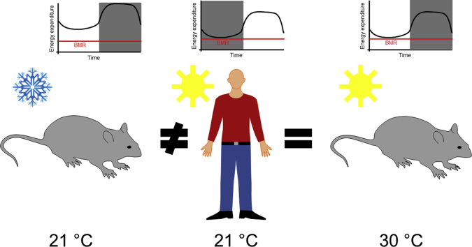
Objectives: The laboratory mouse is presently the most common model for examining mechanisms of human physiology and disease. Housing temperatures can have a large impact on the outcome of such experiments and on their translatability to the human situation. Humans usually create for themselves a thermoneutral environment without cold stress, while laboratory mice under standard conditions (≈20° C) are under constant cold stress. In a well-cited, theoretical paper by Speakman and Keijer in Molecular Metabolism, it was argued that housing mice under close to standard conditions is the optimal way of modeling the human metabolic situation. This tenet was mainly based on the observation that humans usually display average metabolic rates of about 1.6 times basal metabolic rate. The extra heat thereby produced would also be expected to lead to a shift in the 'lower critical temperature' towards lower temperatures.

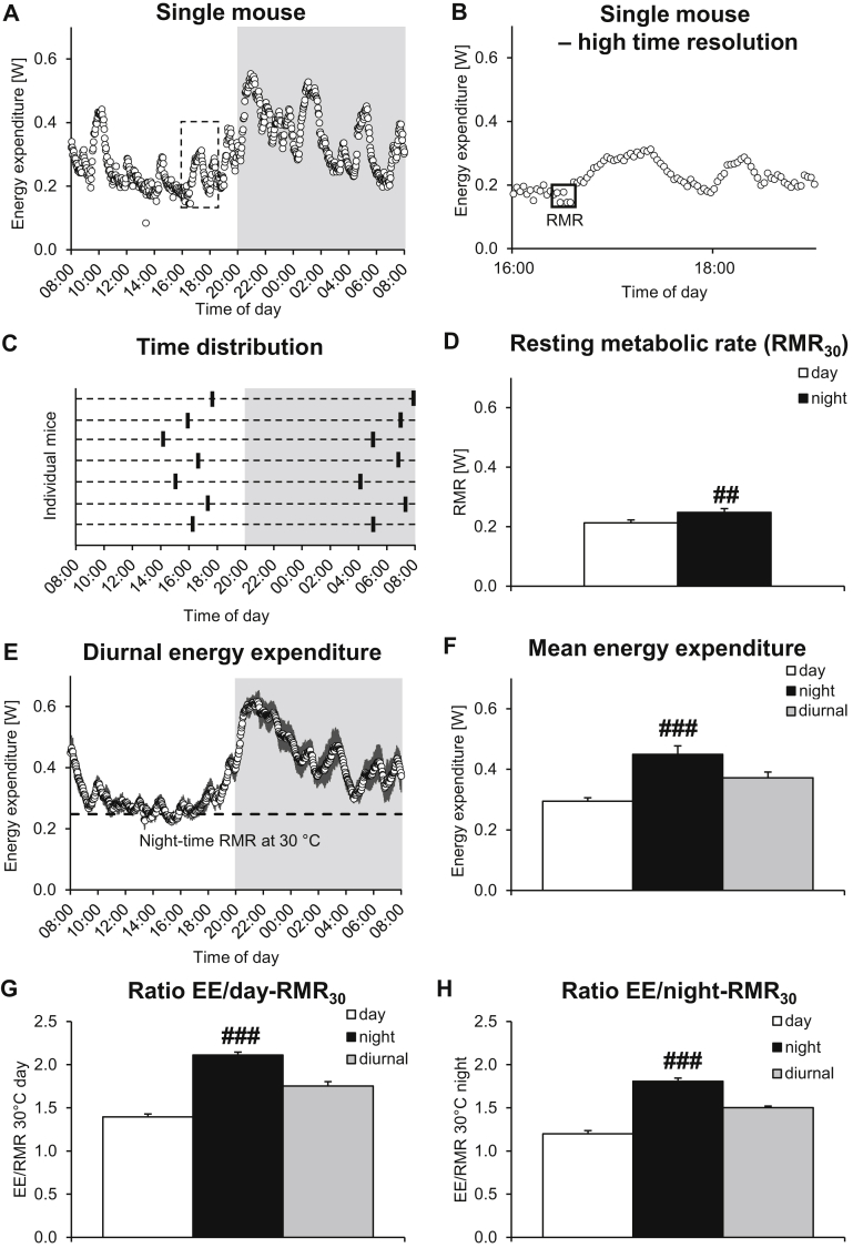
Methods: To examine these tenets experimentally, we performed high time-resolution indirect calorimetry at different environmental temperatures on mice acclimated to different housing temperatures.

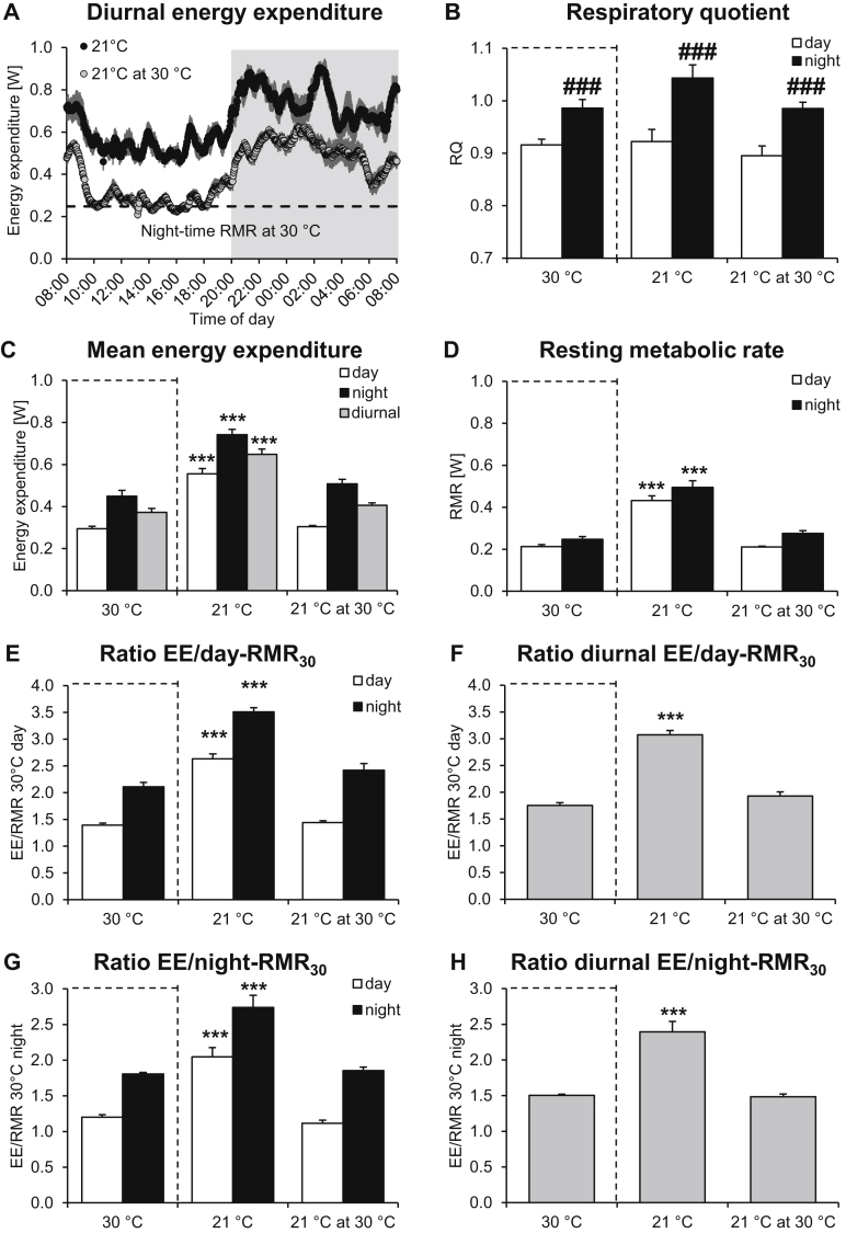
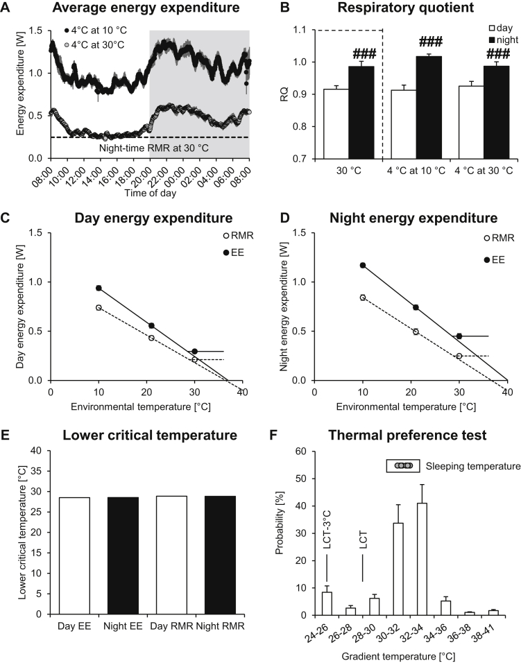
Results: Based on the high time-resolution calorimetry analysis, we found that mice already under thermoneutral conditions display mean diurnal energy expenditure rates 1.8 times higher than basal metabolism, remarkably closely resembling the human situation. At any temperature below thermoneutrality, mice metabolism therefore exceeds the human equivalent: Mice under standard conditions display energy expenditure 3.1 times basal metabolism. The discrepancy to previous conclusions is probably attributable to earlier limitations in establishing true mouse basal metabolic rate, due to low time resolution. We also found that the fact that mean energy expenditure exceeds resting metabolic rate does not move the apparent thermoneutral zone (the lower critical temperature) downwards.

Conclusions: We show that housing mice at thermoneutrality is an advantageous step towards aligning mouse energy metabolism to human energy metabolism.

Keywords: Ambient temperature; Basal metabolic rate; Human; Lower critical temperature; Mouse; Thermoneutral; Thermoregulation.

Graphical abstract

Figure 1

Establishment of the ratio between resting metabolic rate and average energy expenditure in mice at thermoneutrality reveals similarity to human metabolism. To examine the relationship between resting and total metabolism in mice under thermoneutral conditions, male 12-week-old C57BL/6 mice were acclimated to 30 °C for 4 weeks and energy expenditure was recorded with high time-resolution. A. Representative 24 h energy expenditure trace of a single mouse showing phases of higher and lower energy expenditure during both day- and night-time. Gray background indicates dark phase. Box indicates the time-frame shown in the high time-resolution figure in B. B. High time-resolution of a 3 h interval of the representative trace from A showing phases of higher and lower energy expenditure. The lowest 5 consecutive values are indicated and their average was defined as RMR (Box). Note that there were lower single values, but the box represents the lowest 10 min and these were the values that were used for further analysis. C. Time distribution of the lowest 10 min of energy expenditure used for calculation of the resting metabolic rate for the individual mice. Each stippled line represents one mouse. Note the clustering in the end of the dark phase and shortly before the end of the light phase. D. Average resting metabolic rate for day- and night-time. E. Mean diurnal energy expenditure trace of 7 mice. Dashed line indicates the calculated average resting metabolic rate (RMR) during night-time from D. F. Average day, night, and diurnal energy expenditure. G. Ratio between day-time, night-time and diurnal energy expenditure and day-time RMR₃₀. H. Ratio between day-time, night-time and diurnal energy expenditure and night-time RMR₃₀. All values in D–H are the means ± SEM of 7 mice. ## and ### indicates p ≤ 0.01 and 0.001 between day- and night-time by Student's paired t-test (for each mouse); for the group, there was no significant difference between the mean day- and night-time RMR₃₀ (panel D).

Figure 2

In mice housed under standard animal house conditions, energy expenditure does not mimic human conditions. To examine the relationship between resting and total metabolism in mice under standard animal housing conditions, male 12-week-old C57BL/6 mice were acclimated to 21 °C for 4 weeks and energy expenditure was recorded. A. Average energy expenditure trace for 7 mice. The mice were first measured at 21 °C and subsequently at 30 °C. Dashed line indicates the calculated average resting metabolic rate during night-time in the 30 °C-acclimated mice from Figure 1. B. Average respiratory quotient showing typical diurnal rhythmicity. Note that here and in the following graphs, the 30 °C values from Figure 1 are shown for comparison (indicated by dashed boxes). C. Mean day-time, night-time, and diurnal energy expenditure. D. Average day-time and night-time RMR at different temperatures. The RMR₃₀, i.e. the RMR of mice housed under standard conditions (21 °C) but measured acutely at 30 °C (“21 °C at 30 °C”) was used to calculate the ratios shown in E–H. E, F. Ratio between day-time (E), night-time (E) and diurnal (F) energy expenditure and day-time RMR₃₀. G, H. Ratio between day-time (G), night-time (G) and diurnal (H) energy expenditure and night-time RMR₃₀. All values are the means ± SEM of 7 mice. In B, ### indicates p ≤ 0.001 between day- and night-time by Student's paired t-test (for each mouse). Note that statistically significant day–night differences are not indicated in the other graphs. *** indicates p ≤ 0.001 for the values different from those of 30 °C-acclimated mice.

Figure 3

Determination of the lower critical temperature. A. Male 12-week-old C57BL/6 mice were acclimated to 4 °C (after 1 week at 18 °C) for 4 weeks, and energy expenditure was recorded at 10 °C and 30 °C. Average energy expenditure trace for 7 mice. The mice were first measured at 10 °C and subsequently at 30 °C. Dashed line indicates the calculated average resting metabolic rate (RMR₃₀) during night-time in 30 °C-acclimated mice from Figure 1. B. Average respiratory quotient showing typical diurnal rhythmicity. Note that the 30 °C values already presented in Figure 1 are shown for comparison (indicated by dashed box). C, D. Scholander-like plot for day-time (C) and night-time (D) RMR and total EE. Resting metabolism, as well as average energy expenditure, were plotted against the environmental temperature in a Scholander-like plot to examine the effect on lower critical temperature of activity, as compared to inactive resting. Note that the data from 21 °C and 30 °C are from the calculations presented in Figure 1, Figure 2. The horizontal line indicates the metabolism within the thermoneutral zone (30 °C), the regression lines of the 21 °C and 10 °C energy expenditure represent the increased need to produce heat in order to maintain euthermia. The intercept of the 2 lines indicates the lower critical temperature. The regression lines extrapolate to the apparent defended body temperature. E. Calculated lower critical temperature for the different conditions displayed in C and D. Note that different groups of mice were used at each temperature; thus, no individual lower critical temperature values for each mouse could be calculated. F. Thermal preference test. Probability distribution of staying in the indicated temperature zones of a metal temperature gradient is shown, as well as the preferred sleeping temperature (dots). Note that the distribution, but not the sleeping temperature, has already been shown in . It should be noted that 24 °C was the temperature at the end of the gradient box, where the mice initially seemed to seek protection when put into the gradient. LCT indicates the lower critical temperature from E; LCT – 3 °C indicates the preferred temperature as suggested by Speakman and Keijer . All values are the means ± SEM of 7 mice for A–C and 9 mice for F. Note that in C and D, the SEM was generally smaller than the size of the symbols.

References

1. Abreu-Vieira G., Fischer A.W., Mattsson C., de Jong J.M.A., Shabalina I.G., Rydén M. Cidea improves the metabolic profile through expansion of adipose tissue. Nature Communications. 2015;6:7433. - PubMed
1. Cannon B., Nedergaard J. Nonshivering thermogenesis and its adequate measurement in metabolic studies. Journal of Experimental Biology. 2011;214:242–253. - PubMed
1. Dudele A., Rasmussen G.M., Mayntz D., Malte H., Lund S., Wang T. Effects of ambient temperature on glucose tolerance and insulin sensitivity test outcomes in normal and obese C57 male mice. Physiological Reports. 2015;3 - PMC - PubMed
1. Feldmann H.M., Golozoubova V., Cannon B., Nedergaard J. UCP1 ablation induces obesity and abolishes diet-induced thermogenesis in mice exempt from thermal stress by living at thermoneutrality. Cell Metabolism. 2009;9:203–209. - PubMed
1. Ganeshan K., Chawla A. Warming the mouse to model human diseases. Nature Reviews Endocrinology. 2017;13:458–465. - PMC - PubMed
Publication types