Protein-Ligand Blind Docking Using QuickVina-W With Inter-Process Spatio-Temporal Integration

Abstract

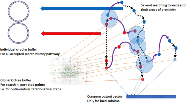
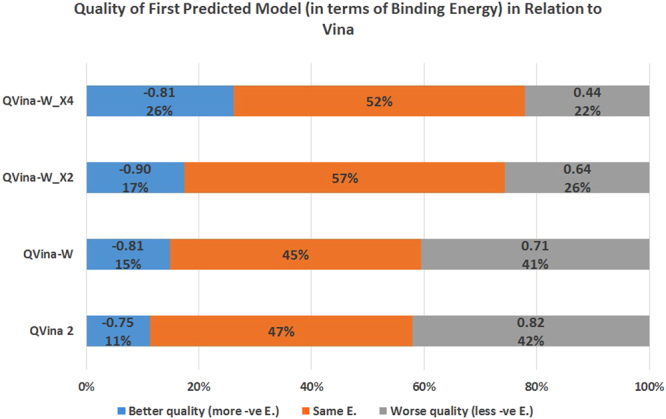
"Virtual Screening" is a common step of in silico drug design, where researchers screen a large library of small molecules (ligands) for interesting hits, in a process known as "Docking". However, docking is a computationally intensive and time-consuming process, usually restricted to small size binding sites (pockets) and small number of interacting residues. When the target site is not known (blind docking), researchers split the docking box into multiple boxes, or repeat the search several times using different seeds, and then merge the results manually. Otherwise, the search time becomes impractically long. In this research, we studied the relation between the search progression and Average Sum of Proximity relative Frequencies (ASoF) of searching threads, which is closely related to the search speed and accuracy. A new inter-process spatio-temporal integration method is employed in Quick Vina 2, resulting in a new docking tool, QuickVina-W, a suitable tool for "blind docking", (not limited in search space size or number of residues). QuickVina-W is faster than Quick Vina 2, yet better than AutoDock Vina. It should allow researchers to screen huge ligand libraries virtually, in practically short time and with high accuracy without the need to define a target pocket beforehand.

Figure 1

Flow chart of the search algorithm. Flow chart of the search algorithm in Vina, QVina 2, and QVina-W respectively from left to right.

Figure 2

Illustration of progression of threads proximity in 2D. (A–C) represent the searching threads while 0, 1, 2, 3, and 4 refer to the time point at which the thread is. The dark area at the lower right corner represents a local minimum.

Figure 3

Overview of the whole tool with both types of buffers. Searching threads are shown in violet solid arrows (for Monte Carlo optimization) and black dotted arrows (for BFGS optimization). End (stop) points are shown as small red/blue spheres. Areas where threads come close to each other are shown as light blue spheres. All history points are continuously added to the circular buffer, while end points are stored in the Octree according to their three-dimensional position. Finally, the local minima are added to the results vector.

Figure 4

Study of search progress of 10GS. (I) Progression of Average of Sum of proximity relative Frequencies (ASoF) of the first 340 time frames. The numbers are averaged over periods of 1000 steps each. The curve shows an initial sharp rising segment and a terminal falling segment (frames 1–12 and 260–340 respectively, both colored in green). Between these segments, a rising trend (frames 13–259, colored in magenta) appears with a slightly shifted small segment (frames 161–210, colored in blue).To investigate and explain the reason of this curve’s features, we mark some representative points with black circles (frames 1, 9, 32, 140, 166, 204, 224, 305, and 338), and show their snapshots in (II). (II) Snapshots of the search progress of ligand-protein complex PDB ID 10GS, using 64 threads. The ligands representing the searching threads are in black. (III) Progression of Frequency of G test pass among all passes. Every point is the sum of G pass among 2000 passes (either G or I pass) from all threads.

Figure 5

Analysis of decision-making process. (A) Progression of decision time, in terms of number of checks taken to pass a potentially significant point, is the sum of checks done in 7500 passed tests. (B) Fractional analysis of decision taking time components. The frequency of success in the Global stage increases with time, while the frequency of success in the Individual stage is stationary.

Figure 6

Normalized Search Time Trend for QVina-W for steps X1, X2, and X4. The curve shift from middle to lower curves is much bigger than the shift from the upper to the middle curves, indicating that the search speed keeps increasing as the search progresses, in an increasing rate.

Figure 7

Progression of G check Sensitivity. The sensitivity of the global checks is shown in relation to time in terms of a unit of 1000 steps of the search process.

Figure 8

Relation between ASoF and Average thread Sensitivity. A plot of both ASOF and average sensitivity in relation to time in term of a unit of 1000 steps. It shows the definite relation between them with Correlation Coefficient r = 0.862.

Figure 9

Quality of first predicted model (in terms of binding energy) of different steps of QVina-W and the previously published version of QVina, in relation to Vina. Binding energy of the first predicted model of the previously published version of QVina(QVina 2), and QVina-W with different steps compared to Vina. The decimal numbers on both sides are the average Binding Energy difference.

Figure 10

RMSD of Vina, QVina 2, and QVina-W. Relative frequency of successes using RMSD to experimental data for both Vina and QVina-W. (A) RMSD distribution of the first mode. (B) First mode success at 2.0 A. (C) RMSD distribution of the best mode. (D) Best mode success at 2.0 A.

Figure 11

Acceleration of QVina 2 and QVina-W (different steps) against Vina. (A) Overall time acceleration for QVina 2 and QVina-W steps X1, X2, X4 against Vina. (B) Normalized overall time acceleration for QVina 2 and QVina-W.

References

1. Walters WP, Stahl MT, Murcko MA. Virtual screening - an overview. Drug Discovery Today. 1998;3:160–178. doi: 10.1016/S1359-6446(97)01163-X. - DOI
1. Shin WH, Seok C. GalaxyDock: protein-ligand docking with flexible protein side-chains. Journal of chemical information and modeling. 2012;52:3225–3232. doi: 10.1021/ci300342z. - DOI - PubMed
1. Ravindranath PA, Forli S, Goodsell DS, Olson AJ, Sanner MF. AutoDockFR: Advances in Protein-Ligand Docking with Explicitly Specified Binding Site Flexibility. Plos Comput Biol. 2015;11:e1004586. doi: 10.1371/journal.pcbi.1004586. - DOI - PMC - PubMed
1. Trott O, Olson AJ. AutoDock Vina: improving the speed and accuracy of docking with a new scoring function, efficient optimization, and multithreading. Journal of computational chemistry. 2010;31:455–461. - PMC - PubMed
1. Wang Z, et al. Comprehensive evaluation of ten docking programs on a diverse set of protein-ligand complexes: the prediction accuracy of sampling power and scoring power. Phys Chem Chem Phys. 2016;18:12964–12975. doi: 10.1039/C6CP01555G. - DOI - PubMed
Publication types