. 2017 Nov 15;12(11):e0187163.
doi: 10.1371/journal.pone.0187163. eCollection 2017.

Low cost and open source multi-fluorescence imaging system for teaching and research in biology and bioengineering

Affiliations

Low cost and open source multi-fluorescence imaging system for teaching and research in biology and bioengineering

Isaac Nuñez et al. PLoS One. .

Abstract

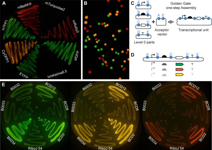
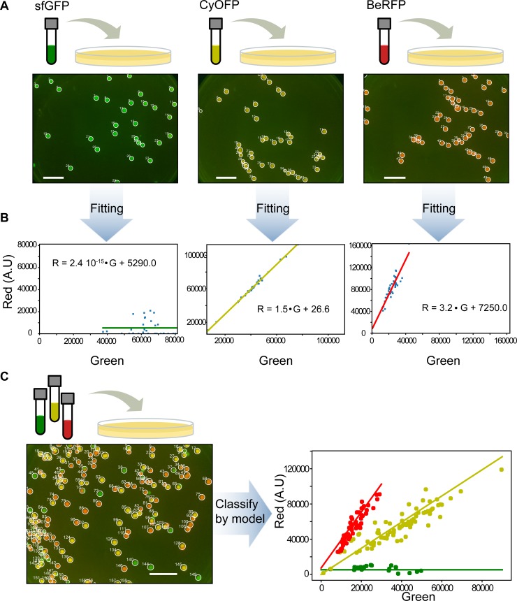
The advent of easy-to-use open source microcontrollers, off-the-shelf electronics and customizable manufacturing technologies has facilitated the development of inexpensive scientific devices and laboratory equipment. In this study, we describe an imaging system that integrates low-cost and open-source hardware, software and genetic resources. The multi-fluorescence imaging system consists of readily available 470 nm LEDs, a Raspberry Pi camera and a set of filters made with low cost acrylics. This device allows imaging in scales ranging from single colonies to entire plates. We developed a set of genetic components (e.g. promoters, coding sequences, terminators) and vectors following the standard framework of Golden Gate, which allowed the fabrication of genetic constructs in a combinatorial, low cost and robust manner. In order to provide simultaneous imaging of multiple wavelength signals, we screened a series of long stokes shift fluorescent proteins that could be combined with cyan/green fluorescent proteins. We found CyOFP1, mBeRFP and sfGFP to be the most compatible set for 3-channel fluorescent imaging. We developed open source Python code to operate the hardware to run time-lapse experiments with automated control of illumination and camera and a Python module to analyze data and extract meaningful biological information. To demonstrate the potential application of this integral system, we tested its performance on a diverse range of imaging assays often used in disciplines such as microbial ecology, microbiology and synthetic biology. We also assessed its potential use in a high school environment to teach biology, hardware design, optics, and programming. Together, these results demonstrate the successful integration of open source hardware, software, genetic resources and customizable manufacturing to obtain a powerful, low cost and robust system for education, scientific research and bioengineering. All the resources developed here are available under open source licenses.


Conflict of interest statement

Competing Interests: Authors TCM and RHP contributed to this work under employment by Backyard Brains, a company that develops and distributes open source scientific equipment. Backyard Brains worked on this project under support of the OpenPlant fund. This does not alter our adherence to PLOS ONE policies on sharing data and materials. Additionally, there are no patents, products in development or marketed products to declare.

Figures

Fig 1
Fig 1. Device general architecture.
(A) Schematic rendering of the device with and without the front lid. (B) lateral view of a longitudinal cross-section of the device showing height control, illumination box and filters. (C) Camera and amber filter holder.
Fig 2
Fig 2. Simultaneous imaging of different fluorescent proteins with single excitation at 470 nm.
(A) CyOFP1, hmKeima8.5, mBeRFP, mRuby2, mTFP1, sfGFP, mTurquoise2, and EYFP, with R0010 promoter and RiboJ 54 insulator-RBS treated with (right) and without (left) IPTG. (B) Representative image showing growing E. coli colonies expressing sfGFP, CyOFP1 and mBeRFP. (C) Schematic representation of Golden Gate one-step assembly for the construction of genetic systems from level 0 parts. (D) Schematic representation of combinations of promoter, ribosome binding sites (RBS), coding DNA sequence (CDS) and terminator that can be assembled with the standardized Golden Gate method. (E) Image of agar plates with streaks of E. coli expressing sfGFP, CyOFP1 and mBeRFP under J23101 promoter and different ribosome binding sites (RBS): BCD12; BCD8; BCD2; RiboJ54; B0034; B0033; and B0032. B0015 terminator was used for all the constructs. No post-editing has been applied to these images; only cropping and alignment.
Fig 3
Fig 3. System testing under different experimental setups.
(A) Image of ISO-GRID permeable membrane used in experiments shown in B to D. Scale bar, 1000 μm. (B) Schematic representation of diffusion assay for E. coli cells producing (“sender cells”) and responding to (“receiver cells”) C6 and C12 homoserine lactones plated on permeable membranes printed with hydrophobics grid lines. (C) Images of a time-lapse experiment of cell responses to C6 and C12 homoserine lactones. Images were taken at 12 and 28 hours after plating. Cells were grown at 37°C outside the device. Vector co-transformation for: strong C12 receiver, pTet_32 LasR + pLas8O; weak C12 receiver, pTet_32 LasR + pLas33O; strong C6 receiver, 1LU2 + pLux34G; weak C6 receiver, 1LU2 + pLux54G; strong C6 sender, Std34BeRFP + pLac34LuxI; weak C6 sender, Std34BeRFP + pLac54LuxI; strong C12 sender, Std34BeRFP + pLac34LasI; weak C12 sender, Std34BeRFP + pLac54LasI. See Table 1 for sequence information. Scale bar, 1000 μm. (D) Images at 48h after plating a mix of C6 and C12 sender cells (expressing mBeRFP, in red) and a mix of C6 and C12 receiver cells expressing sfGFP and CyOFP, respectively. ROH: pTet_32 LasR + pLas8O. (E) Colony-sectoring assay. Strains labelled with CyOFP1, mBeRFP and sfGFP fluorescent proteins seeded on agar LB plates in combinations of two (CyOFP1-mBeRFP, CyOFP1sfGFP and sfGFP-mBeRFP) or three (CyOFP1, mBeRFP and sfGFP) and tracked every 24h for 6 days. No post-editing has been applied to these images; only cropping and alignment. Scale bar, 500 μm.
Fig 4
Fig 4. Colony identification and segmentation from timelapse images.
A) Endpoint timelapse image (see S4 Movie) of a plate with growing colonies of three different strains, each one expressing a different fluorescent protein. Scale bar = 1cm. B) Colony identification (label them with an ID), by getting position in the image and final size. C) Segmentation of regions of interest (ROIs) defined by the standard deviation of the identified blobs. One example of each strain is shown.
Fig 5
Fig 5. Analysis and parameter estimation from identified colonies.
(A) kymograph of the pixel signal in the central slice of an example colony. The x marks show the radius estimated for each time and the red line is the radius value obtained from a fitted area function (also red circles). (B) Colony area curve fitting for some example colonies. Dots are the estimated area from the standard deviation of the blobs and the continuous lines are the model fitting of this values (C) Mean fluorescence intensity signal over time for the example colonies. Lines were obtained by spline smoothing. (D) Colony growth rate estimation from the data for each selected colony. (E) Protein expression rate parameter estimation using the previous data.
Fig 6
Fig 6. Distinguishing different strains by (R,G) color profile.
(A) Timelapse images were taken separately of three strains, each expressing a different fluorescent protein (sfGFP, BeRFP and CyOFP). Figure shows final image (see S5–S7 Movies) with the detected colonies labeled. Scale bar = 1cm. (B) Characteristic linear relationship between red and green channel for each strain/fluorescent protein obtained from each timelapse in A. Each dot is the (R,G) total signal pair of a colony and the straight line is the linear regression. (C) When grown together on the same plate, the characteristic profile obtained could be used to classify the colonies according to strain/fluorescent protein (see S8 Movie). Scale bar = 1 cm.

Similar articles

Cited by

References

    1. Gibney E.'Open-hardware' pioneers push for low-cost lab kit. Nature. 2016;531(7593):147–8. doi: 10.1038/531147a - DOI - PubMed
    1. Baden T, Chagas AM, Gage G, Marzullo T, Prieto-Godino LL, Euler T. Open Labware: 3-D Printing Your Own Lab Equipment. PLOS Biol. 2015;13(3):e1002086 doi: 10.1371/journal.pbio.1002086 - DOI - PMC - PubMed
    1. Pearce JM. Building Research Equipment with Free, Open-Source Hardware. Science. 2012;337(6100):1303–1304. doi: 10.1126/science.1228183 - DOI - PubMed
    1. Pearce J. M. Laboratory equipment: Cut costs with open-source hardware. Nature. 2014; 505 (7485), 618. - PubMed
    1. http://openpcr.org

MeSH terms